change of parameter
(0.003 seconds)
41—50 of 54 matching pages
41: 2.3 Integrals of a Real Variable
…
►Then
…
►Then the series obtained by substituting (2.3.7) into (2.3.1) and integrating formally term by term yields an asymptotic expansion:
…
►When the parameter
is large the contributions from the real and imaginary parts of the integrand in
…However, cancellation does not take place near the endpoints, owing to lack of symmetry, nor in the neighborhoods of zeros of because
changes relatively slowly at these stationary points.
…
►A uniform approximation can be constructed by quadratic change of integration variable:
…
42: 10.17 Asymptotic Expansions for Large Argument
…
►
10.17.1
,
►
10.17.2
…
►
10.17.8
…
►where denotes the variational operator (2.3.6), and the paths of variation are subject to the condition that
changes monotonically.
…
►
10.17.17
…
43: 19.28 Integrals of Elliptic Integrals
44: 28.6 Expansions for Small
…
►
28.6.1
…
►
28.6.4
►
28.6.5
…
►
28.6.8
…
►For the corresponding expansions of for
change
to everywhere in (28.6.26).
…
45: 3.5 Quadrature
…
►
3.5.39
…
►The integral (3.5.39) has the form (3.5.35) if we set , , and .
…
►When is large the integral becomes exponentially small, and application of the quadrature rule of §3.5(viii) is useless.
…
►
3.5.43
.
…
►
3.5.46
,
…
46: Bibliography K
…
►
Connecting Jacobi elliptic functions with different modulus parameters.
Pramana 63 (5), pp. 921–936.
…
►
A vortex filament moving without change of form.
J. Fluid Mech. 112, pp. 397–409.
…
►
Approximation Formulae for Generalized Hypergeometric Functions for Large Values of the Parameters.
J. B. Wolters, Groningen.
…
47: 27.2 Functions
…
►
27.2.3
…
►
27.2.4
…
►
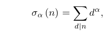
27.2.10
►is the sum of the th powers of the divisors of , where the exponent can be real or complex.
…
►
27.2.14
,
…
48: 28.31 Equations of Whittaker–Hill and Ince
…
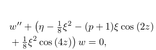
►When is a nonnegative integer, the parameter
can be chosen so that solutions of (28.31.3) are trigonometric polynomials, called Ince polynomials.
…
►
28.31.11
…
►
28.31.18
…
►For change of sign of ,
…
49: 10.21 Zeros
…
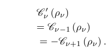
►where is a parameter, then
►
10.21.5
…
►The parameter
may be regarded as a continuous variable and , as functions , of .
…
►
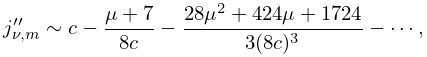
10.21.21
…
►Corresponding uniform approximations for , , , and , are obtained from (10.21.41)–(10.21.44) by changing the symbols , , , , , and to , , , , , and , respectively.
…
50: Bibliography B
…
►
A general program to calculate atomic continuum processes using the R-matrix method.
Comput. Phys. Comm. 8 (3), pp. 149–198.
…
►
Approximating the matrix Fisher and Bingham distributions: Applications to spherical regression and Procrustes analysis.
J. Multivariate Anal. 41 (2), pp. 314–337.
…
►
Mathieu’s Equation for Complex Parameters. Tables of Characteristic Values.
U.S. Government Printing Office, Washington, D.C..
…
►
Table of characteristic values of Mathieu’s equation for large values of the parameter.
J. Washington Acad. Sci. 45 (6), pp. 166–196.
…
