asymptotic expansions for small parameters

SearchAdvancedHelp

(0.005 seconds)

31—40 of 41 matching pages

31: 33.23 Methods of Computation

… ►Use of extended-precision arithmetic increases the radial range that yields accurate results, but eventually other methods must be employed, for example, the asymptotic expansions of §§33.11 and 33.21. … ►Thus the regular solutions can be computed from the power-series expansions (§§33.6, 33.19) for small values of the radii and then integrated in the direction of increasing values of the radii. On the other hand, the irregular solutions of §§33.2(iii) and 33.14(iii) need to be integrated in the direction of decreasing radii beginning, for example, with values obtained from asymptotic expansions (§§33.11 and 33.21). … ►Thompson and Barnett (1985, 1986) and Thompson (2004) use combinations of series, continued fractions, and Padé-accelerated asymptotic expansions (§3.11(iv)) for the analytic continuations of Coulomb functions. ►Noble (2004) obtains double-precision accuracy for $W_{-\eta ,\mu }\left(2\rho \right)$ for a wide range of parameters using a combination of recurrence techniques, power-series expansions, and numerical quadrature; compare (33.2.7). …

32: Bibliography L

… ►

New method to obtain small parameter power series expansions of Mathieu radial and angular functions. Math. Comp. 78 (265), pp. 255–274.

ⓘ

External Links:

ISSN 0025-5718, Document, FullText, MathReview (Junesang Choi), ZentralBlatt

Referenced by:

§28.24, §28.24.

Encodings:

BibTeX

… ►

A note on the uniform asymptotic expansion of integrals with coalescing endpoint and saddle points. J. Phys. A 19 (3), pp. 329–335.

ⓘ

External Links:

ISSN 0305-4470, Document, MathReview (F. W. J. Olver), ZentralBlatt

Referenced by:

§2.4(vi).

Encodings:

BibTeX

… ►

Uniform asymptotic expansions of symmetric elliptic integrals. Constr. Approx. 17 (4), pp. 535–559.

ⓘ

External Links:

ISSN 0176-4276, Document, MathReview (Valdir A. Menegatto), ZentralBlatt

Referenced by:

§19.27(vi).

Encodings:

BibTeX

… ►

Asymptotic expansions of the Whittaker functions for large order parameter. Methods Appl. Anal. 6 (2), pp. 249–256.

ⓘ

Notes:

Dedicated to Richard A. Askey on the occasion of his 65th birthday, Part II

External Links:

ISSN 1073-2772, Pdf, MathReview, ZentralBlatt

Referenced by:

§13.21(i), §13.24(ii).

Encodings:

BibTeX

… ►

Uniform asymptotic expansions at a caustic. Comm. Pure Appl. Math. 19, pp. 215–250.

ⓘ

External Links:

Document, MathReview (Colin Clark), ZentralBlatt

Referenced by:

§36.12(iii), §36.14(i).

Encodings:

BibTeX

…

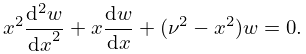
33: 10.45 Functions of Imaginary Order

… ►

10.45.1 $$x^2\frac{d^{2}w}{{dx}^2}+x\frac{dw}{dx}+({\nu }^2-x^2)w=0.$$

ⓘ

Symbols:

$\frac{df}{dx}$: derivative of $f$ with respect to $x$ , $x$: real variable and $\nu$: complex parameter

Referenced by:

§10.45, §10.45

Permalink:

http://dlmf.nist.gov/10.45.E1

Encodings:

pMML, png, TeX

See also:

Annotations for §10.45 and Ch.10

… ►

10.45.6 $${\tilde{I}}_{\nu }\left(x\right)={\left(\frac{\sinh \left(\pi \nu \right)}{\pi \nu }\right)}^{\frac{1}{2}}\cos \left(\nu \ln \left(\frac{1}{2}x\right)-{\gamma }_{\nu }\right)+O\left(x^2\right),$$

ⓘ

Symbols:

$O\left(x\right)$: order not exceeding, $\pi$: the ratio of the circumference of a circle to its diameter, $\cos z$: cosine function, $\sinh z$: hyperbolic sine function, ${\tilde{I}}_{\nu }\left(x\right)$: modified Bessel function of the first kind of imaginary order, $\ln z$: principal branch of logarithm function, $x$: real variable, $\nu$: complex parameter and ${\gamma }_{\nu }$: parameter

Referenced by:

§10.45

Permalink:

http://dlmf.nist.gov/10.45.E6

Encodings:

pMML, png, TeX

See also:

Annotations for §10.45 and Ch.10

… ►In consequence of (10.45.5)–(10.45.7), ${\tilde{I}}_{\nu }\left(x\right)$ and ${\tilde{K}}_{\nu }\left(x\right)$ comprise a numerically satisfactory pair of solutions of (10.45.1) when $x$ is large, and either ${\tilde{I}}_{\nu }\left(x\right)$ and $(1/\pi )\sinh \left(\pi \nu \right){\tilde{K}}_{\nu }\left(x\right)$, or ${\tilde{I}}_{\nu }\left(x\right)$ and ${\tilde{K}}_{\nu }\left(x\right)$, comprise a numerically satisfactory pair when $x$ is small, depending whether $\nu \ne 0$ or $\nu =0$. … ►For properties of ${\tilde{I}}_{\nu }\left(x\right)$ and ${\tilde{K}}_{\nu }\left(x\right)$, including uniform asymptotic expansions for large $\nu$ and zeros, see Dunster (1990a). …

34: 28.4 Fourier Series

… ►

28.4.10 $$\sum _{m=0}^{\mathrm{\infty }}{\left(A_{2m+1}^{2n+1}(q)\right)}^2=1,$$

ⓘ

Symbols:

$m$: integer, $q=h^2$: parameter, $n$: integer and $A_m(q)$: Fourier coefficient

Permalink:

http://dlmf.nist.gov/28.4.E10

Encodings:

pMML, png, TeX

See also:

Annotations for §28.4(iii), §28.4 and Ch.28

►

28.4.11 $$\sum _{m=0}^{\mathrm{\infty }}{\left(B_{2m+1}^{2n+1}(q)\right)}^2=1,$$

ⓘ

Symbols:

$m$: integer, $q=h^2$: parameter, $n$: integer and $B_m(q)$: Fourier coefficient

Permalink:

http://dlmf.nist.gov/28.4.E11

Encodings:

pMML, png, TeX

See also:

Annotations for §28.4(iii), §28.4 and Ch.28

… ►

§28.4(vi) Behavior for Small $q$

… ►For further terms and expansions see Meixner and Schäfke (1954, p. 122) and McLachlan (1947, §3.33). ►

§28.4(vii) Asymptotic Forms for Large $m$

…

35: 18.26 Wilson Class: Continued

… ►

18.26.4_1 $$R_n(y(y+\gamma +\delta +1);\gamma ,\delta ,N)=Q_y(n;\gamma ,\delta ,N),$$

ⓘ

Symbols:

$Q_n(x;\alpha ,\beta ,N)$: Hahn polynomial, $R_n(x;\gamma ,\delta ,N)$: dual Hahn polynomial, $y$: real variable, $N$: positive integer, $\delta$: arbitrary small positive constant and $n$: nonnegative integer

Referenced by:

§18.26(i), Erratum (V1.2.0) Section 18.26

Permalink:

http://dlmf.nist.gov/18.26.E4_1

Encodings:

pMML, png, TeX

Addition (effective with 1.2.0):

This equation was added.

See also:

Annotations for §18.26(i), §18.26(i), §18.26 and Ch.18

… ►

§18.26(v) Asymptotic Approximations

►For asymptotic expansions of Wilson polynomials of large degree see Wilson (1991), and for asymptotic approximations to their largest zeros see Chen and Ismail (1998). ►Koornwinder (2009) rescales and reparametrizes Racah polynomials and Wilson polynomials in such a way that they are continuous in their four parameters, provided that these parameters are nonnegative. Moreover, if one or more of the new parameters becomes zero, then the polynomial descends to a lower family in the Askey scheme.

36: 10.24 Functions of Imaginary Order

… ►

10.24.1 $$x^2\frac{d^{2}w}{{dx}^2}+x\frac{dw}{dx}+(x^2+{\nu }^2)w=0.$$

ⓘ

Symbols:

$\frac{df}{dx}$: derivative of $f$ with respect to $x$ , $x$: real variable and $\nu$: complex parameter

Referenced by:

§10.24, §10.24

Permalink:

http://dlmf.nist.gov/10.24.E1

Encodings:

pMML, png, TeX

See also:

Annotations for §10.24 and Ch.10

… ►

10.24.3 $$\mathrm{\Gamma }\left(1+\mathrm{i}\nu \right)={\left(\frac{\pi \nu }{\sinh \left(\pi \nu \right)}\right)}^{\frac{1}{2}}{\mathrm{e}}^{\mathrm{i}{\gamma }_{\nu }},$$

ⓘ

Symbols:

$\mathrm{\Gamma }\left(z\right)$: gamma function, $\pi$: the ratio of the circumference of a circle to its diameter, $\mathrm{e}$: base of natural logarithm, $\sinh z$: hyperbolic sine function, $\mathrm{i}$: imaginary unit, $\nu$: complex parameter and ${\gamma }_{\nu }$: parameter

Permalink:

http://dlmf.nist.gov/10.24.E3

Encodings:

pMML, png, TeX

See also:

Annotations for §10.24 and Ch.10

… ►Also, in consequence of (10.24.7)–(10.24.9), when $x$ is small either ${\tilde{J}}_{\nu }\left(x\right)$ and $\tanh \left(\frac{1}{2}\pi \nu \right){\tilde{Y}}_{\nu }\left(x\right)$ or ${\tilde{J}}_{\nu }\left(x\right)$ and ${\tilde{Y}}_{\nu }\left(x\right)$ comprise a numerically satisfactory pair depending whether $\nu \ne 0$ or $\nu =0$. … ►For mathematical properties and applications of ${\tilde{J}}_{\nu }\left(x\right)$ and ${\tilde{Y}}_{\nu }\left(x\right)$, including zeros and uniform asymptotic expansions for large $\nu$, see Dunster (1990a). …

37: 18.15 Asymptotic Approximations

… ►Here, and elsewhere in §18.15, $\delta$ is an arbitrary small positive constant. … ►The first term of this expansion also appears in Szegő (1975, Theorem 8.21.7). … ►Here $J_{\nu }\left(z\right)$ denotes the Bessel function (§10.2(ii)), $\mathrm{env}{J}_{\nu }\left(z\right)$ denotes its envelope (§2.8(iv)), and $\delta$ is again an arbitrary small positive constant. … ►For more powerful asymptotic expansions as $n\to \mathrm{\infty }$ in terms of elementary functions that apply uniformly when , $-1+\delta \le t\le 1-\delta$, or , where $t=x/\sqrt{2n+1}$ and $\delta$ is again an arbitrary small positive constant, see §§12.10(i)–12.10(iv) and 12.10(vi). … ►The asymptotic behavior of the classical OP’s as $x\to \pm \mathrm{\infty }$ with the degree and parameters fixed is evident from their explicit polynomial forms; see, for example, (18.2.7) and the last two columns of Table 18.3.1. …

38: 13.20 Uniform Asymptotic Approximations for Large $\mu$

… ►

§13.20(i) Large $\mu$, Fixed $\kappa$

… ►For an extension of (13.20.1) to an asymptotic expansion, together with error bounds, see Olver (1997b, Chapter 10, Ex. 3.4). … ► … ►

§13.20(v) Large $\mu$, Other Expansions

… ►

39: 33.20 Expansions for Small $|ϵ|$

§33.20 Expansions for Small $|ϵ|$

… ►

§33.20(iii) Asymptotic Expansion for the Irregular Solution

… ►

§33.20(iv) Uniform Asymptotic Expansions

►For a comprehensive collection of asymptotic expansions that cover $f(ϵ,\mathrm{\ell };r)$ and $h(ϵ,\mathrm{\ell };r)$ as $ϵ\to 0\pm$ and are uniform in $r$, including unbounded values, see Curtis (1964a, §7). These expansions are in terms of elementary functions, Airy functions, and Bessel functions of orders $2\mathrm{\ell }+1$ and $2\mathrm{\ell }+2$.

40: 13.2 Definitions and Basic Properties

… ►

Kummer’s Equation

… ►The first two standard solutions are: … ►

13.2.6 $$U(a,b,z)\sim z^{-a},$$ $z\to \mathrm{\infty }$, $|\mathrm{ph}z|\le \frac{3}{2}\pi -\delta$,

ⓘ

Defines:

$U(a,b,z)$: Kummer confluent hypergeometric function

Symbols:

$\sim$: asymptotic equality, $\pi$: the ratio of the circumference of a circle to its diameter, $\mathrm{ph}$: phase, $z$: complex variable and $\delta$: small positive constant

Referenced by:

§13.2(i), §13.2(iv)

Permalink:

http://dlmf.nist.gov/13.2.E6

Encodings:

pMML, png, TeX

See also:

Annotations for §13.2(i), §13.2(i), §13.2 and Ch.13

►where $\delta$ is an arbitrary small positive constant. … ►where $\delta$ is an arbitrary small positive constant. …