asymptotic behavior of coefficients

SearchAdvancedHelp

(0.002 seconds)

11—20 of 22 matching pages

11: 2.11 Remainder Terms; Stokes Phenomenon

… ►with … … ►However, to enjoy the resurgence property (§2.7(ii)) we often seek instead expansions in terms of the $F$-functions introduced in §2.11(iii), leaving the connection of the error-function type behavior as an implicit consequence of this property of the $F$-functions. … ► … ►in which …

12: 2.7 Differential Equations

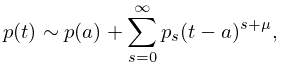
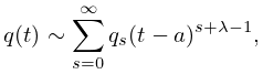
… ►is one at which the coefficients $f(z)$ and $g(z)$ are analytic. … ►Formal solutions are … ►Note that the coefficients in the expansions (2.7.12), (2.7.13) for the “late” coefficients, that is, $a_{s,1}$, $a_{s,2}$ with $s$ large, are the “early” coefficients $a_{j,2}$, $a_{j,1}$ with $j$ small. …See §2.11(v) for other examples. … ►For irregular singularities of nonclassifiable rank, a powerful tool for finding the asymptotic behavior of solutions, complete with error bounds, is as follows: …

13: 2.3 Integrals of a Real Variable

… ►For the Fourier integral … ►Other types of singular behavior in the integrand can be treated in an analogous manner. … ►

As $t\to a+$

2.3.14

$$p(t)\sim p(a)+\sum _{s=0}^{\mathrm{\infty }}{p}_s{(t-a)}^{s+\mu },$$

$$q(t)\sim \sum _{s=0}^{\mathrm{\infty }}{q}_s{(t-a)}^{s+\lambda -1},$$

ⓘ

Symbols:

$\sim$: Poincaré asymptotic expansion, $a$: left endpoint, $p(t)$: real function, $p_s$: coefficients, $q(t)$: function, $q_s$: coefficients, $\lambda$: positive constant and $\mu$: positive constant

Referenced by:

item (b)

Permalink:

http://dlmf.nist.gov/2.3.E14

Encodings:

pMML, pMML, png, png, TeX, TeX

See also:

Annotations for §2.3(iii), §2.3 and Ch.2

and the expansion for $p(t)$ is differentiable. Again $\lambda$ and $\mu$ are positive constants. Also $p_0>0$ (consistent with (a)).

… ►Then … ►

§2.3(vi) Asymptotics of Mellin Transforms

…

14: Bibliography K

… ►

Pascal program for generating tables of $\mathrm{SU}(3)$ Clebsch-Gordan coefficients. Comput. Phys. Comm. 85 (1), pp. 82–88.

ⓘ

External Links:

ISSN 0010-4655, Document, Code, MathReview Entry, ZentralBlatt

Referenced by:

6th item.

Encodings:

BibTeX

… ►

Asymptotic behavior of the solutions of the Painlevé equation of the first kind. Differ. Uravn. 24 (10), pp. 1684–1695 (Russian).

ⓘ

Notes:

In Russian. English translation: Differential Equations 24(1988), no. 10, pp. 1107–1115 (1989)

External Links:

ISSN 0374-0641, MathReview, ZentralBlatt

Referenced by:

§32.11(i).

Encodings:

BibTeX

… ►

Asymptotic approximations for the first incomplete elliptic integral near logarithmic singularity. J. Comput. Appl. Math. 205 (1), pp. 186–206.

ⓘ

External Links:

ISSN 0377-0427, Document, FullText, MathReview (José Luis López), ZentralBlatt

Referenced by:

§19.12, §19.12, §19.36(iv), §19.36(iv).

Encodings:

BibTeX

… ►

Clebsch-Gordan coefficients for $\mathrm{SU}(2)$ and Hahn polynomials. Nieuw Arch. Wisk. (3) 29 (2), pp. 140–155.

ⓘ

External Links:

ISSN 0028-9825, MathReview (Jiří Patera), ZentralBlatt

Referenced by:

§18.38(iii).

Encodings:

BibTeX

… ►

Asymptotic solution of Maxwell’s equations near caustics. Izv. Vuz. Radiofiz. 7, pp. 1049–1056.

ⓘ

Referenced by:

§36.14(i).

Encodings:

BibTeX

…

15: 3.5 Quadrature

… ►The $w_k$ are also known as Christoffel coefficients or Christoffel numbers and they are all positive. The remainder is given by … ►In practical applications the weight function $w(x)$ is chosen to simulate the asymptotic behavior of the integrand as the endpoints are approached. … ►Below we give for the classical orthogonal polynomials the recurrence coefficients ${\alpha }_n$ and ${\beta }_n$ in (3.5.30). These also immediately yield the recurrence coefficients in (3.5.30_5). …

16: 18.2 General Orthogonal Polynomials

… ►Then, with the coefficients (18.2.11_4) associated with the monic OP’s $p_n$, the orthonormal recurrence relation for $q_n$ takes the form … ►The monic and orthonormal OP’s, and their determination via recursion, are more fully discussed in §§3.5(v) and 3.5(vi), where modified recursion coefficients are listed for the classical OP’s in their monic and orthonormal forms. … ►Alternatives for numerical calculation of the recursion coefficients in terms of the moments are discussed in these references, and in §18.40(ii). … ►This says roughly that the series (18.2.25) has the same pointwise convergence behavior as the same series with $p_n(x)=T_n\left(x\right)$, a Chebyshev polynomial of the first kind, see Table 18.3.1. … ►for certain coefficients $a_{n,j}$ with $s,t$ independent of $n$. …

17: 30.11 Radial Spheroidal Wave Functions

… ►

§30.11(iii) Asymptotic Behavior

… ►For asymptotic expansions in negative powers of $z$ see Meixner and Schäfke (1954, p. 293). … ►where ►

30.11.10 $$K_n^m(\gamma )=\frac{\sqrt{\pi }}{2}{\left(\frac{\gamma }{2}\right)}^m\frac{{(-1)}^m{a}_{n,\frac{1}{2}(m-n)}^{-m}({\gamma }^2)}{\mathrm{\Gamma }\left(\frac{3}{2}+m\right)A_n^{-m}({\gamma }^2){\mathrm{𝖯𝗌}}_n^m(0,{\gamma }^2)},$$ $n-m$ even,

ⓘ

Symbols:

$\mathrm{\Gamma }\left(z\right)$: gamma function, $\pi$: the ratio of the circumference of a circle to its diameter, ${\mathrm{𝖯𝗌}}_n^m(x,{\gamma }^2)$: spheroidal wave function of the first kind, $m$: nonnegative integer, $n\ge m$: integer degree, $A_n^m({\gamma }^2)$ , $K_n^m(\gamma )$: connection coefficient, ${\gamma }^2$: real parameter and $a_{n,k}^m({\gamma }^2)$: coefficients

Referenced by:

§30.16(iii)

Permalink:

http://dlmf.nist.gov/30.11.E10

Encodings:

pMML, png, TeX

See also:

Annotations for §30.11(v), §30.11 and Ch.30

… ►

30.11.11 $$K_n^m(\gamma )=\frac{\sqrt{\pi }}{2}{\left(\frac{\gamma }{2}\right)}^{m+1}\frac{{(-1)}^m{a}_{n,\frac{1}{2}(m-n+1)}^{-m}({\gamma }^2)}{\mathrm{\Gamma }\left(\frac{5}{2}+m\right)A_n^{-m}({\gamma }^2)({d{\mathrm{𝖯𝗌}}_n^m(z,{\gamma }^2)/dz|}_{z=0})},$$ $n-m$ odd.

ⓘ

Symbols:

$\mathrm{\Gamma }\left(z\right)$: gamma function, $\pi$: the ratio of the circumference of a circle to its diameter, $\frac{df}{dx}$: derivative of $f$ with respect to $x$ , ${\mathrm{𝖯𝗌}}_n^m(x,{\gamma }^2)$: spheroidal wave function of the first kind, $z$: complex variable, $m$: nonnegative integer, $n\ge m$: integer degree, $A_n^m({\gamma }^2)$ , $K_n^m(\gamma )$: connection coefficient, ${\gamma }^2$: real parameter and $a_{n,k}^m({\gamma }^2)$: coefficients

Referenced by:

§30.16(iii)

Permalink:

http://dlmf.nist.gov/30.11.E11

Encodings:

pMML, png, TeX

See also:

Annotations for §30.11(v), §30.11 and Ch.30

…

18: 18.15 Asymptotic Approximations

§18.15 Asymptotic Approximations

►

§18.15(i) Jacobi

… ►

§18.15(ii) Ultraspherical

… ►The leading coefficients are given by … ►The asymptotic behavior of the classical OP’s as $x\to \pm \mathrm{\infty }$ with the degree and parameters fixed is evident from their explicit polynomial forms; see, for example, (18.2.7) and the last two columns of Table 18.3.1. …

19: 25.11 Hurwitz Zeta Function

… ►

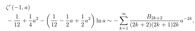
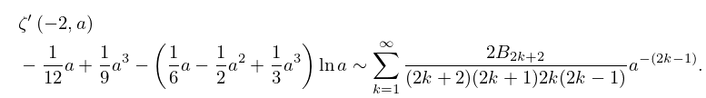
§25.11(xii) $a$-Asymptotic Behavior

… ►As $a\to \mathrm{\infty }$ in the sector , with $s(\ne 1)$ and $\delta$ fixed, we have the asymptotic expansion … ►Similarly, as $a\to \mathrm{\infty }$ in the sector , ►

25.11.44 $${\zeta }^{\prime }(-1,a)-\frac{1}{12}+\frac{1}{4}{a}^2-\left(\frac{1}{12}-\frac{1}{2}a+\frac{1}{2}{a}^2\right)\ln a\sim -\sum _{k=1}^{\mathrm{\infty }}\frac{B_{2k+2}}{(2k+2)(2k+1)2k}{a}^{-2k},$$

ⓘ

Symbols:

$B_n$: Bernoulli numbers, $\zeta (s,a)$: Hurwitz zeta function, $\sim$: Poincaré asymptotic expansion, $\ln z$: principal branch of logarithm function, $k$: nonnegative integer and $a$: real or complex parameter

Keywords:

asymptotic approximation

Source:

Elizalde (1986, (18), p. 349)

Permalink:

http://dlmf.nist.gov/25.11.E44

Encodings:

pMML, png, TeX

See also:

Annotations for §25.11(xii), §25.11 and Ch.25

… ►

25.11.45 $${\zeta }^{\prime }(-2,a)-\frac{1}{12}a+\frac{1}{9}{a}^3-\left(\frac{1}{6}a-\frac{1}{2}{a}^2+\frac{1}{3}{a}^3\right)\ln a\sim \sum _{k=1}^{\mathrm{\infty }}\frac{2B_{2k+2}}{(2k+2)(2k+1)2k(2k-1)}{a}^{-(2k-1)}.$$

ⓘ

Symbols:

$B_n$: Bernoulli numbers, $\zeta (s,a)$: Hurwitz zeta function, $\sim$: Poincaré asymptotic expansion, $\ln z$: principal branch of logarithm function, $k$: nonnegative integer and $a$: real or complex parameter

Keywords:

asymptotic approximation

Source:

Elizalde (1986, (19), p. 350)

Permalink:

http://dlmf.nist.gov/25.11.E45

Encodings:

pMML, png, TeX

See also:

Annotations for §25.11(xii), §25.11 and Ch.25

…

20: 15.12 Asymptotic Approximations

§15.12 Asymptotic Approximations

►

§15.12(i) Large Variable

►For the asymptotic behavior of $𝐅(a,b;c;z)$ as $z\to \mathrm{\infty }$ with $a$, $b$, $c$ fixed, combine (15.2.2) with (15.8.2) or (15.8.8). ►

§15.12(ii) Large $c$

… ►For other extensions, see Wagner (1986), Temme (2003) and Temme (2015, Chapters 12 and 28).