applied to generalized hypergeometric functions

(0.017 seconds)

11—20 of 50 matching pages

11: 2.10 Sums and Sequences

… ►For extensions of the Euler–Maclaurin formula to functions

f(x)

with singularities at

x=a

x=n

(or both) see Sidi (2004, 2012b, 2012a). … ►The asymptotic behavior of entire functions defined by Maclaurin series can be approached by converting the sum into a contour integral by use of the residue theorem and applying the methods of §§2.4 and 2.5. … ►Hence … ►For generalizations and other examples see Olver (1997b, Chapter 8), Ford (1960), and Berndt and Evans (1984). … ►However, if

r

is finite and

f(z)

has algebraic or logarithmic singularities on

|z|=r

, then Darboux’s method is usually easier to apply. …

12: 16.8 Differential Equations

… ► … ►

§16.8(ii) The Generalized Hypergeometric Differential Equation

… ►In Letessier et al. (1994) examples are discussed in which the generalized hypergeometric function satisfies a differential equation that is of order 1 or even 2 less than might be expected. … ►(Note that the generalized hypergeometric functions on the right-hand side are polynomials in

z_{0}

.) … ►In this reference it is also explained that in general when

q>1

no simple representations in terms of generalized hypergeometric functions are available for the fundamental solutions near

z=1

. …

13: 13.14 Definitions and Basic Properties

… ►Standard solutions are: … ►In general

M_{\kappa,\mu}\left(z\right)

and

W_{\kappa,\mu}\left(z\right)

are many-valued functions of

z

with branch points at

z=0

and

z=\infty

. The principal branches correspond to the principal branches of the functions

z^{\frac{1}{2}+\mu}

and

U\left(\tfrac{1}{2}+\mu-\kappa,1+2\mu,z\right)

on the right-hand sides of the equations (13.14.2) and (13.14.3); compare §4.2(i). … ►Although

M_{\kappa,\mu}\left(z\right)

does not exist when

2\mu=-1,-2,-3,\dots

, many formulas containing

M_{\kappa,\mu}\left(z\right)

continue to apply in their limiting form. … ►Also, unless specified otherwise

M_{\kappa,\mu}\left(z\right)

and

W_{\kappa,\mu}\left(z\right)

are assumed to have their principal values. …

14: 19.16 Definitions

… ►

§19.16(ii) $R_{-a}\left(\mathbf{b};\mathbf{z}\right)$

►All elliptic integrals of the form (19.2.3) and many multiple integrals, including (19.23.6) and (19.23.6_5), are special cases of a multivariate hypergeometric function …which is homogeneous and of degree

-a

in the

z

’s, and unchanged when the same permutation is applied to both sets of subscripts

1,\dots,n

. … ►For generalizations and further information, especially representation of the

R

-function as a Dirichlet average, see Carlson (1977b). …

15: 15.9 Relations to Other Functions

… ►

§15.9(i) Orthogonal Polynomials

… ►

Jacobi

… ►

Legendre

… ►

Meixner

… ►The following formulas apply with principal branches of the hypergeometric functions, associated Legendre functions, and fractional powers. …

16: Bibliography S

… ►

J. B. Seaborn (1991) Hypergeometric Functions and Their Applications. Texts in Applied Mathematics, Vol. 8, Springer-Verlag, New York.

ⓘ

External Links:: ISBN 0-387-97558-6, MathReview (Wolfgang Bühring), ZentralBlatt
Referenced by:: Erratum (V1.2.0) Section 18.39.
Encodings:: BibTeX

… ►

L. J. Slater (1966) Generalized Hypergeometric Functions. Cambridge University Press, Cambridge.

ⓘ

External Links:: ISBN 9780521090612, MathReview (S. C. van Veen), ZentralBlatt
Referenced by:: Ch.15, §16.2(iii), §16.4(ii), §16.4(iii), §16.4(v), Ch.16, §17.1, §17.4(i), Ch.17.
Encodings:: BibTeX

… ►

D. Slepian (1964) Prolate spheroidal wave functions, Fourier analysis and uncertainity. IV. Extensions to many dimensions; generalized prolate spheroidal functions. Bell System Tech. J. 43, pp. 3009–3057.

ⓘ

External Links:: ISSN 0005-8580, MathReview (J. Meixner), ZentralBlatt
Referenced by:: §30.12.
Encodings:: BibTeX

… ►

C. Snow (1952) Hypergeometric and Legendre Functions with Applications to Integral Equations of Potential Theory. National Bureau of Standards Applied Mathematics Series, No. 19, U. S. Government Printing Office, Washington, D.C..

ⓘ

External Links:: MathReview, ZentralBlatt
Referenced by:: §13.23(iv), Ch.14, §31.3(iii).
Encodings:: BibTeX

… ►

K. Srinivasa Rao (1981) Computation of angular momentum coefficients using sets of generalized hypergeometric functions. Comput. Phys. Comm. 22 (2-3), pp. 297–302.

ⓘ

External Links:: Document
Referenced by:: §34.13.
Encodings:: BibTeX

…

17: Bibliography M

… ►

N. Michel and M. V. Stoitsov (2008) Fast computation of the Gauss hypergeometric function with all its parameters complex with application to the Pöschl-Teller-Ginocchio potential wave functions. Comput. Phys. Comm. 178 (7), pp. 535–551.

ⓘ

External Links:: ISSN 0010-4655, Document, FullText, MathReview Entry, ZentralBlatt
Referenced by:: §15.19(i), §15.19(i).
Encodings:: BibTeX

… ►

C. Micu and E. Papp (2005) Applying

q

-Laguerre polynomials to the derivation of

q

-deformed energies of oscillator and Coulomb systems. Romanian Reports in Physics 57 (1), pp. 25–34.

ⓘ

Referenced by:: §17.17.
Encodings:: BibTeX

… ►

A. R. Miller and R. B. Paris (2011) Euler-type transformations for the generalized hypergeometric function

{}_{r+2}F_{r+1}(x)

. Z. Angew. Math. Phys. 62 (1), pp. 31–45.

ⓘ

External Links:: ISSN 0044-2275, Document, FullText, MathReview (Mridula Garg), ZentralBlatt
Referenced by:: §16.6, §16.6.
Encodings:: BibTeX

►

A. R. Miller (1997) A class of generalized hypergeometric summations. J. Comput. Appl. Math. 87 (1), pp. 79–85.

ⓘ

External Links:: ISSN 0377-0427, Document, MathReview, ZentralBlatt
Referenced by:: §16.10.
Encodings:: BibTeX

►

A. R. Miller (2003) On a Kummer-type transformation for the generalized hypergeometric function

{}_{2}F_{2}

. J. Comput. Appl. Math. 157 (2), pp. 507–509.

ⓘ

External Links:: ISSN 0377-0427, Document, MathReview Entry, ZentralBlatt
Referenced by:: §16.6.
Encodings:: BibTeX

…

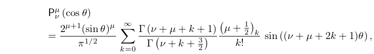
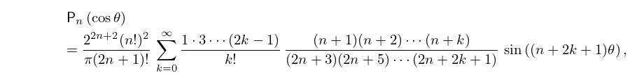
18: 14.13 Trigonometric Expansions

§14.13 Trigonometric Expansions

… ►

14.13.1

\mathsf{P}^{\mu}_{\nu}\left(\cos\theta\right)=\frac{2^{\mu+1}(\sin\theta)^{\mu% }}{\pi^{1/2}}\*\sum_{k=0}^{\infty}\frac{\Gamma\left(\nu+\mu+k+1\right)}{\Gamma% \left(\nu+k+\frac{3}{2}\right)}\frac{{\left(\mu+\frac{1}{2}\right)_{k}}}{k!}\*% \sin\left((\nu+\mu+2k+1)\theta\right),

ⓘ

Symbols:: $\Gamma\left(\NVar{z}\right)$ : gamma function, $\mathsf{P}^{\NVar{\mu}}_{\NVar{\nu}}\left(\NVar{x}\right)$ : Ferrers function of the first kind, ${\left(\NVar{a}\right)_{\NVar{n}}}$ : Pochhammer’s symbol (or shifted factorial), $\pi$ : the ratio of the circumference of a circle to its diameter, $\cos\NVar{z}$ : cosine function, $!$ : factorial (as in $n!$ ), $\sin\NVar{z}$ : sine function, $\mu$ : general order, $\nu$ : general degree and $0<\theta<\pi$ : variable
Source:: Volkmer (2021)
A&S Ref:: 8.7.1
Referenced by:: §14.13, Erratum (V1.1.3) for Equations (14.13.1), (14.13.2)
Permalink:: http://dlmf.nist.gov/14.13.E1
Encodings:: pMML, png, TeX
See also:: Annotations for §14.13 and Ch.14

►

14.13.2

\mathsf{Q}^{\mu}_{\nu}\left(\cos\theta\right)=\pi^{1/2}2^{\mu}(\sin\theta)^{% \mu}\*\sum_{k=0}^{\infty}\frac{\Gamma\left(\nu+\mu+k+1\right)}{\Gamma\left(\nu% +k+\frac{3}{2}\right)}\frac{{\left(\mu+\frac{1}{2}\right)_{k}}}{k!}\*\cos\left% ((\nu+\mu+2k+1)\theta\right).

ⓘ

Symbols:: $\Gamma\left(\NVar{z}\right)$ : gamma function, $\mathsf{Q}^{\NVar{\mu}}_{\NVar{\nu}}\left(\NVar{x}\right)$ : Ferrers function of the second kind, ${\left(\NVar{a}\right)_{\NVar{n}}}$ : Pochhammer’s symbol (or shifted factorial), $\pi$ : the ratio of the circumference of a circle to its diameter, $\cos\NVar{z}$ : cosine function, $!$ : factorial (as in $n!$ ), $\sin\NVar{z}$ : sine function, $\mu$ : general order, $\nu$ : general degree and $0<\theta<\pi$ : variable
Source:: Cohl et al. (2021, Theorem 6.2)
A&S Ref:: 8.7.2
Referenced by:: §14.13, Erratum (V1.1.3) for Equations (14.13.1), (14.13.2)
Permalink:: http://dlmf.nist.gov/14.13.E2
Encodings:: pMML, png, TeX
See also:: Annotations for §14.13 and Ch.14

… ►

14.13.3

\mathsf{P}_{n}\left(\cos\theta\right)=\frac{2^{2n+2}(n!)^{2}}{\pi(2n+1)!}\*% \sum_{k=0}^{\infty}\frac{1\cdot 3\cdots(2k-1)}{k!}\*\frac{(n+1)(n+2)\cdots(n+k% )}{(2n+3)(2n+5)\cdots(2n+2k+1)}\*\sin\left((n+2k+1)\theta\right),

ⓘ

Symbols:: $\pi$ : the ratio of the circumference of a circle to its diameter, $\cos\NVar{z}$ : cosine function, $!$ : factorial (as in $n!$ ), $\mathsf{P}_{\NVar{\nu}}\left(\NVar{x}\right)=\mathsf{P}^{0}_{\nu}\left(x\right)$ : Ferrers function of the first kind, $\sin\NVar{z}$ : sine function, $n$ : nonnegative integer and $0<\theta<\pi$ : variable
A&S Ref:: 8.7.3
Permalink:: http://dlmf.nist.gov/14.13.E3
Encodings:: pMML, png, TeX
See also:: Annotations for §14.13 and Ch.14

►

14.13.4

\mathsf{Q}_{n}\left(\cos\theta\right)=\frac{2^{2n+1}(n!)^{2}}{(2n+1)!}\*\sum_{% k=0}^{\infty}\frac{1\cdot 3\cdots(2k-1)}{k!}\*\frac{(n+1)(n+2)\cdots(n+k)}{(2n% +3)(2n+5)\cdots(2n+2k+1)}\*\cos\left((n+2k+1)\theta\right),

ⓘ

Symbols:: $\cos\NVar{z}$ : cosine function, $!$ : factorial (as in $n!$ ), $\mathsf{Q}_{\NVar{\nu}}\left(\NVar{x}\right)=\mathsf{Q}^{0}_{\nu}\left(x\right)$ : Ferrers function of the second kind, $n$ : nonnegative integer and $0<\theta<\pi$ : variable
A&S Ref:: 8.7.4
Permalink:: http://dlmf.nist.gov/14.13.E4
Encodings:: pMML, png, TeX
See also:: Annotations for §14.13 and Ch.14

…

19: Bibliography D

… ►

C. de Boor (2001) A Practical Guide to Splines. Revised edition, Applied Mathematical Sciences, Vol. 27, Springer-Verlag, New York.

ⓘ

External Links:: ISBN 0-387-95366-3, MathReview (Gerlind Plonka-Hoch), ZentralBlatt
Referenced by:: §3.11(vi).
Encodings:: BibTeX

… ►

K. Dilcher, L. Skula, and I. Sh. Slavutskiǐ (1991) Bernoulli Numbers. Bibliography (1713–1990). Queen’s Papers in Pure and Applied Mathematics, Vol. 87, Queen’s University, Kingston, ON.

ⓘ

Notes:: A frequently updated version, with links to reviews, exists online
External Links:: Online version, MathReview, ZentralBlatt
Referenced by:: Ch.24.
Encodings:: BibTeX

… ►

K. Dilcher (1987b) Irreducibility of certain generalized Bernoulli polynomials belonging to quadratic residue class characters. J. Number Theory 25 (1), pp. 72–80.

ⓘ

External Links:: ISSN 0022-314X, Document, MathReview (T. Metsänkylä)
Referenced by:: §24.12(iii).
Encodings:: BibTeX

… ►

K. Dilcher (2002) Bernoulli Numbers and Confluent Hypergeometric Functions. In Number Theory for the Millennium, I (Urbana, IL, 2000), pp. 343–363.

ⓘ

External Links:: ISBN 1-56881-126-8, MathReview (Arnold M. Adelberg), ZentralBlatt
Referenced by:: §24.16(iii).
Encodings:: BibTeX

… ►

T. M. Dunster (2014) Olver’s error bound methods applied to linear ordinary differential equations having a simple turning point. Anal. Appl. (Singap.) 12 (4), pp. 385–402.

ⓘ

External Links:: ISSN 0219-5305, Document, Link, MathReview (Thomas Mbah Acho), ZentralBlatt
Referenced by:: 5th item, §14.32.
Encodings:: BibTeX

…

20: 14.21 Definitions and Basic Properties

… ►

P^{\pm\mu}_{\nu}\left(z\right)

and

\boldsymbol{Q}^{\mu}_{\nu}\left(z\right)

exist for all values of

\nu

\mu

, and

z

, except possibly

z=\pm 1

and

\infty

, which are branch points (or poles) of the functions, in general. … … ►

§14.21(iii) Properties

… ►This includes, for example, the Wronskian relations (14.2.7)–(14.2.11); hypergeometric representations (14.3.6)–(14.3.10) and (14.3.15)–(14.3.20); results for integer orders (14.6.3)–(14.6.5), (14.6.7), (14.6.8), (14.7.6), (14.7.7), and (14.7.11)–(14.7.16); behavior at singularities (14.8.7)–(14.8.16); connection formulas (14.9.11)–(14.9.16); recurrence relations (14.10.3)–(14.10.7). The generating function expansions (14.7.19) (with

\mathsf{P}

replaced by

P

) and (14.7.22) apply when

|h|<\min\left|z\pm\left(z^{2}-1\right)^{1/2}\right|

; (14.7.21) (with

\mathsf{P}