…
►
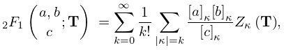
35.7.1
, ;
.
…
►
Case
►
35.7.3
…
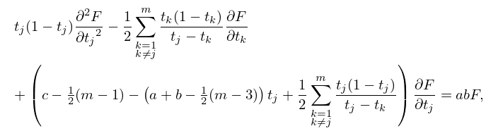
►Subject to the conditions (a)–(c), the function
is the unique solution of each partial differential equation
►
35.7.9
…
…
►Then (
2.4.1) is valid in any closed sector with vertex
and properly interior to
.
…
►
(b)
ranges along a ray or over an annular sector
, , where
, , and .
converges at absolutely and uniformly with respect to .
…
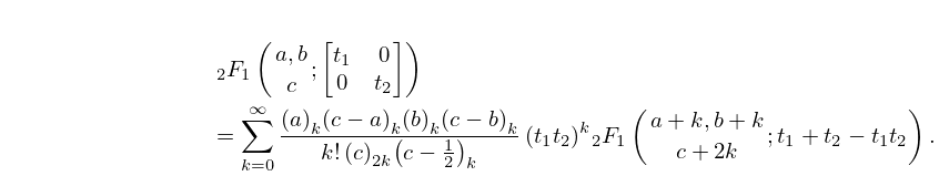
►Higher coefficients
in (
2.4.15) can be found from (
2.3.18) with
,
, and
replaced by
.
…The last reference also includes examples, as do
Olver (1997b, Chapter 4),
Wong (1989, Chapter 2), and
Bleistein and Handelsman (1975, Chapter 7).
…
►with
and
chosen so that the zeros of
correspond to the zeros
, say, of the quadratic
.
…
…
►To code a message by this method, we replace each letter by two digits, say
,
,
,
, and divide the message into pieces of convenient length smaller than the public value
.
…
…
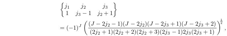
►If any lower argument in a
symbol is
,
, or
, then the
symbol has a simple algebraic form.
…
►
34.5.5
►
34.5.6
►
34.5.7
…
►
34.5.13
…
…
►The main functions treated in this chapter are the eigenvalues
,
,
,
, the Lamé functions
,
,
,
, and the Lamé polynomials
,
,
,
,
,
,
,
.
…
►Other notations that have been used are as follows:
Ince (1940a) interchanges
with
.
The relation to the Lamé functions
,
of
Jansen (1977) is given by
…
►
►where the positive factors
and
are determined by
…
…
►
§22.9(ii) Typical Identities of Rank 2
…
►These identities are
cyclic in the sense that each of the indices
in the first product of, for example, the form
are
simultaneously permuted in the cyclic order:
;
.
…
►
22.9.11
►
22.9.12
…
►
22.9.21
…
