Legendre elliptic integrals

SearchAdvancedHelp

(0.018 seconds)

31—40 of 76 matching pages

31: 19.12 Asymptotic Approximations

§19.12 Asymptotic Approximations

… ►

19.12.1 $$K\left(k\right)=\sum _{m=0}^{\mathrm{\infty }}\frac{{\left(\frac{1}{2}\right)}_m{\left(\frac{1}{2}\right)}_m}{m!m!}k_{}^{\prime }{}_{}{}^{2m}\left(\ln \left(\frac{1}{k^{\prime }}\right)+d(m)\right),$$ ,

ⓘ

Symbols:

${\left(a\right)}_n$: Pochhammer’s symbol (or shifted factorial), $K\left(k\right)$: Legendre’s complete elliptic integral of the first kind, $!$: factorial (as in $n!$), $\ln z$: principal branch of logarithm function, $m$: nonnegative integer, $k$: real or complex modulus, $k^{\prime }$: complementary modulus and $d(m)$: function

Referenced by:

§19.12

Permalink:

http://dlmf.nist.gov/19.12.E1

Encodings:

pMML, png, TeX

See also:

Annotations for §19.12 and Ch.19

►

19.12.2 $$E\left(k\right)=1+\frac{1}{2}\sum _{m=0}^{\mathrm{\infty }}\frac{{\left(\frac{1}{2}\right)}_m{\left(\frac{3}{2}\right)}_m}{{\left(2\right)}_{m}m!}k_{}^{\prime }{}_{}{}^{2m+2}\left(\ln \left(\frac{1}{k^{\prime }}\right)+d(m)-\frac{1}{(2m+1)(2m+2)}\right),$$ ,

ⓘ

Symbols:

${\left(a\right)}_n$: Pochhammer’s symbol (or shifted factorial), $E\left(k\right)$: Legendre’s complete elliptic integral of the second kind, $!$: factorial (as in $n!$), $\ln z$: principal branch of logarithm function, $m$: nonnegative integer, $k$: real or complex modulus, $k^{\prime }$: complementary modulus and $d(m)$: function

Referenced by:

§19.12

Permalink:

http://dlmf.nist.gov/19.12.E2

Encodings:

pMML, png, TeX

See also:

Annotations for §19.12 and Ch.19

… ►

19.12.4 $$(1-{\alpha }^2)\mathrm{\Pi }({\alpha }^2,k)=\left(\ln \frac{4}{k^{\prime }}\right)\left(1+O\left(k_{}^{\prime }{}_{}{}^2\right)\right)-{\alpha }^2{R}_C(1,1-{\alpha }^2),$$ ,

ⓘ

Symbols:

$O\left(x\right)$: order not exceeding, $R_C(x,y)$: Carlson’s combination of inverse circular and inverse hyperbolic functions, $\mathrm{\Pi }({\alpha }^2,k)$: Legendre’s complete elliptic integral of the third kind, $\ln z$: principal branch of logarithm function, $k$: real or complex modulus, $k^{\prime }$: complementary modulus and ${\alpha }^2$: real or complex parameter

Referenced by:

§19.12

Permalink:

http://dlmf.nist.gov/19.12.E4

Encodings:

pMML, png, TeX

See also:

Annotations for §19.12 and Ch.19

►

19.12.5 $$(1-{\alpha }^2)\mathrm{\Pi }({\alpha }^2,k)=\left(\ln \left(\frac{4}{k^{\prime }}\right)-R_C(1,1-{\alpha }^{-2})\right)\left(1+O\left(k_{}^{\prime }{}_{}{}^2\right)\right),$$ .

ⓘ

Symbols:

$O\left(x\right)$: order not exceeding, $R_C(x,y)$: Carlson’s combination of inverse circular and inverse hyperbolic functions, $\mathrm{\Pi }({\alpha }^2,k)$: Legendre’s complete elliptic integral of the third kind, $\ln z$: principal branch of logarithm function, $k$: real or complex modulus, $k^{\prime }$: complementary modulus and ${\alpha }^2$: real or complex parameter

Referenced by:

§19.12

Permalink:

http://dlmf.nist.gov/19.12.E5

Encodings:

pMML, png, TeX

See also:

Annotations for §19.12 and Ch.19

…

32: 22.14 Integrals

… ►

22.14.16 $${\int }_0^{K\left(k\right)}\ln \left(\mathrm{sn}(t,k)\right)dt=-\frac{\pi }{4}{K}^{\prime }\left(k\right)-\frac{1}{2}K\left(k\right)\ln k,$$

ⓘ

Symbols:

$\mathrm{sn}(z,k)$: Jacobian elliptic function, $\pi$: the ratio of the circumference of a circle to its diameter, $K^{\prime }\left(k\right)$: Legendre’s complementary complete elliptic integral of the first kind, $K\left(k\right)$: Legendre’s complete elliptic integral of the first kind, $dx$: differential of $x$ , $\int$: integral, $\ln z$: principal branch of logarithm function and $k$: modulus

Referenced by:

Erratum (V1.0.28) for Equations (22.14.16), (22.14.17)

Permalink:

http://dlmf.nist.gov/22.14.E16

Encodings:

pMML, png, TeX

Correction (effective with 1.0.28):

Originally, a factor of $\pi$ was missing from the term containing the $\frac{1}{4}{K}^{\prime }\left(k\right)$.

Suggested 2020-08-06 by Fred Hucht

See also:

Annotations for §22.14(iv), §22.14 and Ch.22

►

22.14.17 $${\int }_0^{K\left(k\right)}\ln \left(\mathrm{cn}(t,k)\right)dt=-\frac{\pi }{4}{K}^{\prime }\left(k\right)+\frac{1}{2}K\left(k\right)\ln \left(k^{\prime }/k\right),$$

ⓘ

Symbols:

$\mathrm{cn}(z,k)$: Jacobian elliptic function, $\pi$: the ratio of the circumference of a circle to its diameter, $K^{\prime }\left(k\right)$: Legendre’s complementary complete elliptic integral of the first kind, $K\left(k\right)$: Legendre’s complete elliptic integral of the first kind, $dx$: differential of $x$ , $\int$: integral, $\ln z$: principal branch of logarithm function, $k$: modulus and $k^{\prime }$: complementary modulus

Referenced by:

Erratum (V1.0.28) for Equations (22.14.16), (22.14.17)

Permalink:

http://dlmf.nist.gov/22.14.E17

Encodings:

pMML, png, TeX

Correction (effective with 1.0.28):

Originally, a factor of $\pi$ was missing from the term containing the $\frac{1}{4}{K}^{\prime }\left(k\right)$.

Suggested 2020-08-06 by Fred Hucht

See also:

Annotations for §22.14(iv), §22.14 and Ch.22

►

22.14.18 $${\int }_0^{K\left(k\right)}\ln \left(\mathrm{dn}(t,k)\right)dt=\frac{1}{2}K\left(k\right)\ln k^{\prime }.$$

ⓘ

Symbols:

$\mathrm{dn}(z,k)$: Jacobian elliptic function, $K\left(k\right)$: Legendre’s complete elliptic integral of the first kind, $dx$: differential of $x$ , $\int$: integral, $\ln z$: principal branch of logarithm function, $k$: modulus and $k^{\prime }$: complementary modulus

Permalink:

http://dlmf.nist.gov/22.14.E18

Encodings:

pMML, png, TeX

See also:

Annotations for §22.14(iv), §22.14 and Ch.22

…

33: 22.4 Periods, Poles, and Zeros

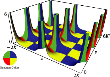
… ►For example, the poles of $\mathrm{sn}(z,k)$, abbreviated as $\mathrm{sn}$ in the following tables, are at $z=2mK+(2n+1)\mathrm{i}{K}^{\prime }$. … ►Figure 22.4.1 illustrates the locations in the $z$-plane of the poles and zeros of the three principal Jacobian functions in the rectangle with vertices $0$, $2K$, $2K+2\mathrm{i}{K}^{\prime }$, $2\mathrm{i}{K}^{\prime }$. … ►The set of points $z=mK+n\mathrm{i}{K}^{\prime }$, $m,n\in \mathbb{Z}$, comprise the lattice for the 12 Jacobian functions; all other lattice unit cells are generated by translation of the fundamental unit cell by $mK+n\mathrm{i}{K}^{\prime }$, where again $m,n\in \mathbb{Z}$. … ►This half-period will be plus or minus a member of the triple $K,\mathrm{i}{K}^{\prime },K+\mathrm{i}{K}^{\prime }$; the other two members of this triple are quarter periods of $\mathrm{p}\mathrm{q}(z,k)$. … ►For example, $\mathrm{sn}(z+K,k)=\mathrm{cd}(z,k)$. …

34: 29.17 Other Solutions

… ►

29.17.1 $$F(z)=E(z){\int }_{\mathrm{i}{K}^{\prime }}^z\frac{du}{{(E(u))}^2}.$$

ⓘ

Symbols:

$K^{\prime }\left(k\right)$: Legendre’s complementary complete elliptic integral of the first kind, $dx$: differential of $x$ , $\mathrm{i}$: imaginary unit, $\int$: integral, $z$: complex variable and $k$: real parameter

Permalink:

http://dlmf.nist.gov/29.17.E1

Encodings:

pMML, png, TeX

See also:

Annotations for §29.17(i), §29.17 and Ch.29

…

35: 19.25 Relations to Other Functions

… ►

§19.25(i) Legendre’s Integrals as Symmetric Integrals

… ►

19.25.2 $$\mathrm{\Pi }({\alpha }^2,k)-K\left(k\right)=\frac{1}{3}{\alpha }^2{R}_J(0,k_{}^{\prime }{}_{}{}^2,1,1-{\alpha }^2).$$

ⓘ

Symbols:

$R_J(x,y,z,p)$: symmetric elliptic integral of third kind, $K\left(k\right)$: Legendre’s complete elliptic integral of the first kind, $\mathrm{\Pi }({\alpha }^2,k)$: Legendre’s complete elliptic integral of the third kind, $k$: real or complex modulus, $k^{\prime }$: complementary modulus and ${\alpha }^2$: real or complex parameter

Referenced by:

§19.12, §19.25(i), §19.6(i)

Permalink:

http://dlmf.nist.gov/19.25.E2

Encodings:

pMML, png, TeX

See also:

Annotations for §19.25(i), §19.25 and Ch.19

… ►Thus the five permutations induce five transformations of Legendre’s integrals (and also of the Jacobian elliptic functions). … ►

§19.25(iii) Symmetric Integrals as Legendre’s Integrals

… ►

19.25.25 $${(z-x)}^{3/2}{R}_D(x,y,z)=(3/k^2)(F(\varphi ,k)-E(\varphi ,k)),$$

ⓘ

Symbols:

$R_D(x,y,z)$: elliptic integral symmetric in only two variables, $F(\varphi ,k)$: Legendre’s incomplete elliptic integral of the first kind, $E(\varphi ,k)$: Legendre’s incomplete elliptic integral of the second kind, $\varphi$: real or complex argument and $k$: real or complex modulus

Referenced by:

§19.25(iii)

Permalink:

http://dlmf.nist.gov/19.25.E25

Encodings:

pMML, png, TeX

See also:

Annotations for §19.25(iii), §19.25 and Ch.19

…

36: 23.6 Relations to Other Functions

… ►

23.6.18 $$e_1=\frac{K^2}{3{\omega }_1^2}(1+k_{}^{\prime }{}_{}{}^2),$$

ⓘ

Symbols:

$e_j$: Weierstrass lattice roots, $K\left(k\right)$: Legendre’s complete elliptic integral of the first kind, $𝕃$: lattice, ${\omega }_1$, ${\omega }_3$, ${\omega }_2=-{\omega }_1-{\omega }_3$: lattice generators, $k$: modulus and $k^{\prime }$: complementary modulus

A&S Ref:

18.9.1

Referenced by:

§23.6(ii)

Permalink:

http://dlmf.nist.gov/23.6.E18

Encodings:

pMML, png, TeX

See also:

Annotations for §23.6(ii), §23.6 and Ch.23

►

23.6.19 $$e_2=\frac{K^2}{3{\omega }_1^2}(k^2-k_{}^{\prime }{}_{}{}^2),$$

ⓘ

Symbols:

$e_j$: Weierstrass lattice roots, $K\left(k\right)$: Legendre’s complete elliptic integral of the first kind, $𝕃$: lattice, ${\omega }_1$, ${\omega }_3$, ${\omega }_2=-{\omega }_1-{\omega }_3$: lattice generators, $k$: modulus and $k^{\prime }$: complementary modulus

A&S Ref:

18.9.2

Permalink:

http://dlmf.nist.gov/23.6.E19

Encodings:

pMML, png, TeX

See also:

Annotations for §23.6(ii), §23.6 and Ch.23

►

23.6.20 $$e_3=-\frac{K^2}{3{\omega }_1^2}(1+k^2).$$

ⓘ

Symbols:

$e_j$: Weierstrass lattice roots, $K\left(k\right)$: Legendre’s complete elliptic integral of the first kind, $𝕃$: lattice, ${\omega }_1$, ${\omega }_3$, ${\omega }_2=-{\omega }_1-{\omega }_3$: lattice generators and $k$: modulus

A&S Ref:

18.9.3

Referenced by:

§23.6(ii)

Permalink:

http://dlmf.nist.gov/23.6.E20

Encodings:

pMML, png, TeX

See also:

Annotations for §23.6(ii), §23.6 and Ch.23

… ►

23.6.27 $$\zeta \left(z|{𝕃}_1\right)-\zeta \left(z+2K|{𝕃}_1\right)+\zeta \left(2K|{𝕃}_1\right)=\mathrm{ns}(z,k),$$

ⓘ

Symbols:

$\mathrm{ns}(z,k)$: Jacobian elliptic function, $\zeta \left(z\right)$ (= $\zeta \left(z|𝕃\right)$ = $\zeta (z;g_2,g_3)$): Weierstrass zeta function, $K\left(k\right)$: Legendre’s complete elliptic integral of the first kind, $𝕃$: lattice, $z$: complex and $k$: modulus

Referenced by:

§23.6(ii), §23.6(ii)

Permalink:

http://dlmf.nist.gov/23.6.E27

Encodings:

pMML, png, TeX

See also:

Annotations for §23.6(ii), §23.6 and Ch.23

►

23.6.28 $$\zeta \left(z|{𝕃}_2\right)-\zeta \left(z+2K|{𝕃}_2\right)+\zeta \left(2K|{𝕃}_2\right)=\mathrm{ds}(z,k),$$

ⓘ

Symbols:

$\mathrm{ds}(z,k)$: Jacobian elliptic function, $\zeta \left(z\right)$ (= $\zeta \left(z|𝕃\right)$ = $\zeta (z;g_2,g_3)$): Weierstrass zeta function, $K\left(k\right)$: Legendre’s complete elliptic integral of the first kind, $𝕃$: lattice, $z$: complex and $k$: modulus

Permalink:

http://dlmf.nist.gov/23.6.E28

Encodings:

pMML, png, TeX

See also:

Annotations for §23.6(ii), §23.6 and Ch.23

…

37: 23.4 Graphics

… ►

§23.4(i) Real Variables

… ►

►►

Figure 23.4.6: $\sigma (x;0,g_3)$ for $-5\le x\le 5$, $g_3$ = 0. … Magnify

►

►►

Figure 23.4.7: $\mathrm{\wp }\left(x\right)$ with ${\omega }_1=K\left(k\right)$, ${\omega }_3=\mathrm{i}{K}^{\prime }\left(k\right)$ for $0\le x\le 9$, $k^2$ = 0. … Magnify

►

§23.4(ii) Complex Variables

… ►

►

►

Figure 23.4.8: $\mathrm{\wp }\left(x+\mathrm{i}y\right)$ with ${\omega }_1=K\left(k\right)$, ${\omega }_3=\mathrm{i}{K}^{\prime }\left(k\right)$ for $-2K\left(k\right)\le x\le 2K\left(k\right)$, $0\le y\le 6K^{\prime }\left(k\right)$, $k^2=0.9$. … Magnify 3D Help

…

38: 19.30 Lengths of Plane Curves

… ►

19.30.3 $$s/a=E(\varphi ,k)=R_F(c-1,c-k^2,c)-\frac{1}{3}{k}^2{R}_D(c-1,c-k^2,c),$$

ⓘ

Symbols:

$R_D(x,y,z)$: elliptic integral symmetric in only two variables, $R_F(x,y,z)$: symmetric elliptic integral of first kind, $E(\varphi ,k)$: Legendre’s incomplete elliptic integral of the second kind, $\varphi$: real or complex argument, $k$: real or complex modulus and $s$: arclength

Referenced by:

§19.30(i)

Permalink:

http://dlmf.nist.gov/19.30.E3

Encodings:

pMML, png, TeX

See also:

Annotations for §19.30(i), §19.30 and Ch.19

… ►

19.30.5 $$L(a,b)=4aE\left(k\right)=8a{R}_G(0,b^2/a^2,1)=8R_G(0,a^2,b^2)=8ab{R}_G(0,a^{-2},b^{-2}),$$

ⓘ

Symbols:

$R_G(x,y,z)$: symmetric elliptic integral of second kind, $E\left(k\right)$: Legendre’s complete elliptic integral of the second kind, $k$: real or complex modulus and $L(a,b)$: length

Referenced by:

§19.15, §19.24(i), §19.30(i), §19.33(i), §19.9(i)

Permalink:

http://dlmf.nist.gov/19.30.E5

Encodings:

pMML, png, TeX

See also:

Annotations for §19.30(i), §19.30 and Ch.19

… ►

19.30.6 $$\frac{\partial s}{\partial (1/k)}=\sqrt{a^2-b^2}F(\varphi ,k)=\sqrt{a^2-b^2}{R}_F(c-1,c-k^2,c),$$ $k^2=(a^2-b^2)/(a^2+\lambda )$, $c={\csc }^2\varphi$.

ⓘ

Symbols:

$R_F(x,y,z)$: symmetric elliptic integral of first kind, $\csc z$: cosecant function, $F(\varphi ,k)$: Legendre’s incomplete elliptic integral of the first kind, $\frac{\partial f}{\partial x}$: partial derivative of $f$ with respect to $x$ , $\partial x$: partial differential of $x$ , $\varphi$: real or complex argument, $k$: real or complex modulus and $s$: arclength

Referenced by:

§19.30(i)

Permalink:

http://dlmf.nist.gov/19.30.E6

Encodings:

pMML, png, TeX

See also:

Annotations for §19.30(i), §19.30 and Ch.19

… ►

19.30.12 $$s=aF(\varphi ,1/\sqrt{2}),$$ $\varphi =\arcsin \sqrt{2/(q+1)}=\arccos \left(\tan \theta \right)$.

ⓘ

Symbols:

$F(\varphi ,k)$: Legendre’s incomplete elliptic integral of the first kind, $\arccos z$: arccosine function, $\arcsin z$: arcsine function, $\tan z$: tangent function, $\varphi$: real or complex argument, $q$ and $s$: arclength

Permalink:

http://dlmf.nist.gov/19.30.E12

Encodings:

pMML, png, TeX

See also:

Annotations for §19.30(iii), §19.30 and Ch.19

… ►

19.30.13 $$P=4\sqrt{2a^2}{R}_F(0,1,2)=\sqrt{2a^2}\times \mathrm{5.24411\hspace{0.33em}51}\mathrm{\dots }=4aK\left(1/\sqrt{2}\right)=a\times \mathrm{7.41629\hspace{0.33em}87}\mathrm{\dots }.$$

ⓘ

Symbols:

$R_F(x,y,z)$: symmetric elliptic integral of first kind, $K\left(k\right)$: Legendre’s complete elliptic integral of the first kind and $P$: length

Notes:

For more digits see OEIS Sequence A064853; see also Sloane (2003).

Permalink:

http://dlmf.nist.gov/19.30.E13

Encodings:

pMML, png, TeX

See also:

Annotations for §19.30(iii), §19.30 and Ch.19

…

39: 19.37 Tables

§19.37 Tables

… ► …

40: 22.20 Methods of Computation

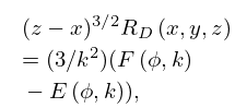
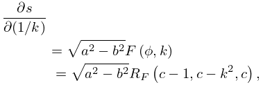
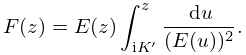
… ►This formula for $\mathrm{dn}$ becomes unstable near $x=K$. If only the value of $\mathrm{dn}(x,k)$ at $x=K$ is required then the exact value is in the table 22.5.1. … ►If $k,k^{\prime }$ are given with $k^2+k_{}^{\prime }{}_{}{}^2=1$ and , then $K,K^{\prime }$ can be found from … ►Jacobi’s epsilon function can be computed from its representation (22.16.30) in terms of theta functions and complete elliptic integrals; compare §20.14. … ►