Julia%20sets

SearchAdvancedHelp

(0.002 seconds)

21—30 of 605 matching pages

21: 26.10 Integer Partitions: Other Restrictions

… ► $p(\in S,n)$ denotes the number of partitions of $n$ into parts taken from the set $S$. The set $\{n\ge 1|n\equiv \pm j(modk)\}$ is denoted by $A_{j,k}$. The set $\{2,3,4,\mathrm{\dots }\}$ is denoted by $T$. … ►

26.10.14 $$p(𝒟2,\in T,n)=p(\in A_{2,5},n),$$ $T=\{2,3,4,\mathrm{\dots }\}$,

ⓘ

Symbols:

$\in$: element of, $p(\mathrm{condition},n)$: restricted number of partitions of $n$ , $n$: nonnegative integer, $A_{j,k}$: set and $T$: set

Referenced by:

§26.10(iv)

Permalink:

http://dlmf.nist.gov/26.10.E14

Encodings:

pMML, png, TeX

See also:

Annotations for §26.10(iv), §26.10 and Ch.26

… ►

26.10.16 $$p(𝒟,n)\sim \frac{{\mathrm{e}}^{\pi \sqrt{n/3}}}{{(768n^3)}^{1/4}},$$ $n\to \mathrm{\infty }$.

ⓘ

Symbols:

$\sim$: asymptotic equality, $\pi$: the ratio of the circumference of a circle to its diameter, $\mathrm{e}$: base of natural logarithm, $p(\mathrm{condition},n)$: restricted number of partitions of $n$ and $n$: nonnegative integer

A&S Ref:

24.2.2

Permalink:

http://dlmf.nist.gov/26.10.E16

Encodings:

pMML, png, TeX

See also:

Annotations for §26.10(v), §26.10 and Ch.26

…

22: 6.16 Mathematical Applications

… ►Hence if $x=\pi /(2n)$ and $n\to \mathrm{\infty }$, then the limiting value of $S_n(x)$ overshoots $\frac{1}{4}\pi$ by approximately 18%. Similarly if $x=\pi /n$, then the limiting value of $S_n(x)$ undershoots $\frac{1}{4}\pi$ by approximately 10%, and so on. … ►

►►

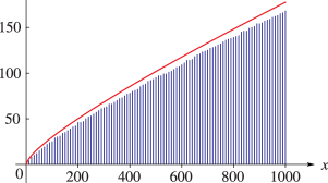
Figure 6.16.2: The logarithmic integral $\mathrm{li}\left(x\right)$, together with vertical bars indicating the value of $\pi (x)$ for $x=10,20,\mathrm{\dots },1000$. Magnify

23: 32.8 Rational Solutions

… ►

32.8.3 $$w(z;3)=\frac{3z^2}{z^3+4}-\frac{6z^2(z^3+10)}{z^6+20z^3-80},$$

ⓘ

Symbols:

$z$: real

Permalink:

http://dlmf.nist.gov/32.8.E3

Encodings:

pMML, png, TeX

See also:

Annotations for §32.8(ii), §32.8 and Ch.32

►

32.8.4 $$w(z;4)=-\frac{1}{z}+\frac{6z^2(z^3+10)}{z^6+20z^3-80}-\frac{9z^5(z^3+40)}{z^9+60z^6+11200}.$$

ⓘ

Symbols:

$z$: real

Permalink:

http://dlmf.nist.gov/32.8.E4

Encodings:

pMML, png, TeX

See also:

Annotations for §32.8(ii), §32.8 and Ch.32

… ►

$$Q_3(z)=z^6+20z^3-80,$$

… ►In the general case assume $\gamma \delta \ne 0$, so that as in §32.2(ii) we may set $\gamma =1$ and $\delta =-1$. … ►In the general case assume $\delta \ne 0$, so that as in §32.2(ii) we may set $\delta =-\frac{1}{2}$. …

24: 7.8 Inequalities

… ►

7.8.2 $x\ge 0$,

ⓘ

Symbols:

$𝖬\left(x\right)$: Mills’ ratio, $\pi$: the ratio of the circumference of a circle to its diameter and $x$: real variable

A&S Ref:

7.1.13

Referenced by:

§7.8

Permalink:

http://dlmf.nist.gov/7.8.E2

Encodings:

pMML, png, TeX

See also:

Annotations for §7.8 and Ch.7

… ►

7.8.5 $x\ge 0$.

ⓘ

Symbols:

$𝖬\left(x\right)$: Mills’ ratio and $x$: real variable

Referenced by:

§7.8

Permalink:

http://dlmf.nist.gov/7.8.E5

Encodings:

pMML, png, TeX

See also:

Annotations for §7.8 and Ch.7

… ►The function $F\left(x\right)/\sqrt{1-{\mathrm{e}}^{-2x^2}}$ is strictly decreasing for $x>0$. … ►

7.8.8 $x>0$.

ⓘ

Symbols:

$\pi$: the ratio of the circumference of a circle to its diameter, $\mathrm{erf}z$: error function, $\mathrm{e}$: base of natural logarithm and $x$: real variable

Source:

Pólya (1949, (1.5))

Referenced by:

§7.8, Erratum (V1.0.17) for Equation (7.8.8)

Permalink:

http://dlmf.nist.gov/7.8.E8

Encodings:

pMML, png, TeX

Addition (effective with 1.0.17):

This inequality was added. It is Pólya (1949, (1.5)). Note that it is a special case of (8.10.11).

Suggested by Roberto Iacono

See also:

Annotations for §7.8 and Ch.7

25: 11.14 Tables

… ►

Zhang and Jin (1996) tabulates ${𝐇}_n\left(x\right)$ and ${𝐋}_n\left(x\right)$ for $n=-4(1)3$ and $x=0(1)20$ to 8D or 7S.

… ►

Abramowitz and Stegun (1964, Chapter 12) tabulates ${\int }_0^x(I_0\left(t\right)-{𝐋}_0\left(t\right))dt$ and $(2/\pi ){\int }_x^{\mathrm{\infty }}{t}^{-1}{𝐇}_0\left(t\right)dt$ for $x=0(.1)5$ to 5D or 7D; ${\int }_0^x({𝐇}_0\left(t\right)-Y_0\left(t\right))dt-(2/\pi )\ln x$, ${\int }_0^x(I_0\left(t\right)-{𝐋}_0\left(t\right))dt-(2/\pi )\ln x$, and ${\int }_x^{\mathrm{\infty }}{t}^{-1}({𝐇}_0\left(t\right)-Y_0\left(t\right))dt$ for $x^{-1}=0(.01)0.2$ to 6D.

…

26: 10.3 Graphics

… ►

►

►

Figure 10.3.14: $H_5^{(1)}\left(x+\mathrm{i}y\right)$, $-20\le x\le 10$, $-4\le y\le 4$. … Magnify 3D Help

… ►

►

►

Figure 10.3.16: $H_{5.5}^{(1)}\left(x+\mathrm{i}y\right)$, $-20\le x\le 10$, $-4\le y\le 4$. … Magnify 3D Help

… ►

►►

Figure 10.3.17: ${\tilde{J}}_{1/2}\left(x\right)$, ${\tilde{Y}}_{1/2}\left(x\right)$, $0.01\le x\le 10$. Magnify

…

27: 36 Integrals with Coalescing Saddles

…

28: Gergő Nemes

… ►As of September 20, 2021, Nemes performed a complete analysis and acted as main consultant for the update of the source citation and proof metadata for every formula in Chapter 25 Zeta and Related Functions. …

29: Wolter Groenevelt

… ►As of September 20, 2022, Groenevelt performed a complete analysis and acted as main consultant for the update of the source citation and proof metadata for every formula in Chapter 18 Orthogonal Polynomials. …

30: 33.24 Tables

… ►

Abramowitz and Stegun (1964, Chapter 14) tabulates $F_0(\eta ,\rho )$, $G_0(\eta ,\rho )$, $F_0^{\prime }(\eta ,\rho )$, and $G_0^{\prime }(\eta ,\rho )$ for $\eta =0.5(.5)20$ and $\rho =1(1)20$, 5S; $C_0\left(\eta \right)$ for $\eta =0(.05)3$, 6S.

…