Gauss transformations
(0.002 seconds)
21—30 of 42 matching pages
21: 15.14 Integrals
§15.14 Integrals
►The Mellin transform of the hypergeometric function of negative argument is given by … ►Fourier transforms of hypergeometric functions are given in Erdélyi et al. (1954a, §§1.14 and 2.14). Laplace transforms of hypergeometric functions are given in Erdélyi et al. (1954a, §4.21), Oberhettinger and Badii (1973, §1.19), and Prudnikov et al. (1992a, §3.37). …Hankel transforms of hypergeometric functions are given in Oberhettinger (1972, §1.17) and Erdélyi et al. (1954b, §8.17). …22: 20.11 Generalizations and Analogs
…
►
§20.11(i) Gauss Sum
►For relatively prime integers with and even, the Gauss sum is defined by …If both are positive, then allows inversion of its arguments as a modular transformation (compare (23.15.3) and (23.15.4)): … … ►Similar identities can be constructed for , , and . …23: 16.16 Transformations of Variables
§16.16 Transformations of Variables
►§16.16(i) Reduction Formulas
… ►§16.16(ii) Other Transformations
… ►For quadratic transformations of Appell functions see Carlson (1976).24: Bibliography G
…
►
Stable computation of high order Gauss quadrature rules using discretization for measures in radiation transfer.
J. Quant. Spectrosc. Radiat. Transfer 68 (2), pp. 213–223.
…
►
Werke. Band II.
pp. 436–447 (German).
…
►
Construction of Gauss-Christoffel quadrature formulas.
Math. Comp. 22, pp. 251–270.
…
►
Gauss quadrature approximations to hypergeometric and confluent hypergeometric functions.
J. Comput. Appl. Math. 139 (1), pp. 173–187.
…
►
Calculation of Gauss quadrature rules.
Math. Comp. 23 (106), pp. 221–230.
…
25: Bibliography M
…
►
Explicit error terms for asymptotic expansions of Stieltjes transforms.
J. Inst. Math. Appl. 22 (2), pp. 129–145.
…
►
Fast computation of the Gauss hypergeometric function with all its parameters complex with application to the Pöschl-Teller-Ginocchio potential wave functions.
Comput. Phys. Comm. 178 (7), pp. 535–551.
…
►
Bäcklund transformations and solution hierarchies for the third Painlevé equation.
Stud. Appl. Math. 98 (2), pp. 139–194.
…
►
A -analog of the Gauss summation theorem for hypergeometric series in
.
Adv. in Math. 72 (1), pp. 59–131.
►
A -analog of a Whipple’s transformation for hypergeometric series in
.
Adv. Math. 108 (1), pp. 1–76.
…
26: 15.10 Hypergeometric Differential Equation
…
►
…
►
…
►(b) If equals , and , then fundamental solutions in the neighborhood of are given by and
…
►The three pairs of fundamental solutions given by (15.10.2), (15.10.4), and (15.10.6) can be transformed into 18 other solutions by means of (15.8.1), leading to a total of 24 solutions known as Kummer’s solutions.
►
15.10.11
…
27: 15.9 Relations to Other Functions
…
►
15.9.7
…
►The Jacobi transform is defined as
…with inverse
…
…
►Any hypergeometric function for which a quadratic transformation exists can be expressed in terms of associated Legendre functions or Ferrers functions.
…
28: 15.6 Integral Representations
…
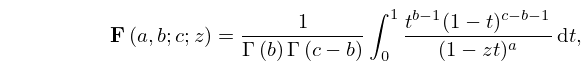
►The function (not ) has the following integral representations:
►
15.6.1
; .
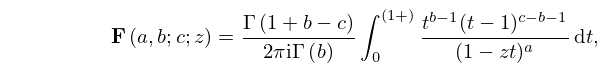
►
15.6.2
; , .
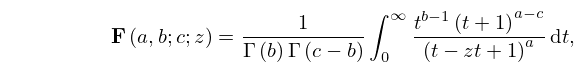
►
15.6.2_5
; .
…
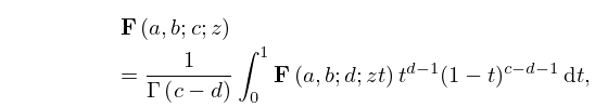
►
15.6.8
; .
…
29: 9.17 Methods of Computation
…
►Among the integral representations of the Airy functions the Stieltjes transform (9.10.18) furnishes a way of computing in the complex plane, once values of this function can be generated on the positive real axis.
…
►The second method is to apply generalized Gauss–Laguerre quadrature (§3.5(v)) to the integral (9.5.8).
…
30: 18.38 Mathematical Applications
…
►It has elegant structures, including -soliton solutions, Lax pairs, and Bäcklund transformations.
While the Toda equation is an important model of nonlinear systems, the special functions of mathematical physics are usually regarded as solutions to linear equations.
…
►For the generalized hypergeometric function see (16.2.1).
…
►
