Euler–Poisson–Darboux equation

SearchAdvancedHelp

(0.003 seconds)

11—20 of 622 matching pages

11: 31.8 Solutions via Quadratures

§31.8 Solutions via Quadratures

… ►the Hermite–Darboux method (see Whittaker and Watson (1927, pp. 570–572)) can be applied to construct solutions of (31.2.1) expressed in quadratures, as follows. … ►The variables $\lambda$ and $\nu$ are two coordinates of the associated hyperelliptic (spectral) curve $\mathrm{\Gamma }:{\nu }^2={\prod }_{j=1}^{2g+1}(\lambda -{\lambda }_j)$. … ►The curve $\mathrm{\Gamma }$ reflects the finite-gap property of Equation (31.2.1) when the exponent parameters satisfy (31.8.1) for $m_j\in \mathbb{Z}$. …For more details see Smirnov (2002). …

12: 14.31 Other Applications

… ►

§14.31(i) Toroidal Functions

►Applications of toroidal functions include expansion of vacuum magnetic fields in stellarators and tokamaks (van Milligen and López Fraguas (1994)), analytic solutions of Poisson’s equation in channel-like geometries (Hoyles et al. (1998)), and Dirichlet problems with toroidal symmetry (Gil et al. (2000)). … ►

§14.31(ii) Conical Functions

… ►

§14.31(iii) Miscellaneous

►Many additional physical applications of Legendre polynomials and associated Legendre functions include solution of the Helmholtz equation, as well as the Laplace equation, in spherical coordinates (Temme (1996b)), quantum mechanics (Edmonds (1974)), and high-frequency scattering by a sphere (Nussenzveig (1965)). …

13: 1.15 Summability Methods

… ►

Poisson Kernel

… ►

Poisson Kernel

… ►is the Poisson integral of $f(t)$. … ► …

14: 18.18 Sums

… ►

§18.18(vii) Poisson Kernels

►See (18.2.41) for the Poisson kernel in case of general OP’s. ►

Laguerre

… ►

Hermite

… ►For the Poisson kernel of Jacobi polynomials (the Bailey formula) see Bailey (1938). …

15: Errata

… ►

The following additions were made in Chapter 1:

• New subsections, 1.2(v) Matrices, Vectors, Scalar Products, and Norms and 1.2(vi) Square Matrices, with Equations (1.2.27)–(1.2.77).

• The title of this section was changed from “Determinants” to “Determinants, Linear Operators, and Spectral Expansions”. An extra paragraph just below (1.3.7). New subsection, 1.3(iv) Matrices as Linear Operators, with Equations (1.3.20), (1.3.21).

• In 1.4(v), three new paragraphs on Stieltjes integrals/measure, with Equations (1.4.23_1)–(1.4.23_3).

• In Subsection 1.8(i), the title of the paragraph “Bessel’s Inequality” was changed to “Parseval’s Formula”. We give the relation between the real and the complex coefficients, and include more general versions of Parseval’s Formula, Equations (1.8.6_1), (1.8.6_2). The title of Subsection 1.8(iv) was changed from “Transformations” to “Poisson’s Summation Formula”, and we added an extra remark just below (1.8.14).

• New subsection, 1.10(xi) Generating Functions, with Equations (1.10.26)–(1.10.29).

• New subsection, 1.13(viii) Eigenvalues and Eigenfunctions: Sturm-Liouville and Liouville forms, with Equations (1.13.26)–(1.13.31).

• Another form of Parseval’s formula, (1.14.7_5).

• We include several extra remarks and Equations (1.16.3_5), (1.16.9_5). New subsection, 1.16(ix) References for Section 1.16.

• Two extra paragraphs in Subsection 1.17(ii) Integral Representations, with Equations (1.17.12_1), (1.17.12_2); Subsection 1.17(iv) Mathematical Definitions is almost completely rewritten.

• An entire new section, 1.18 Linear Second Order Differential Operators and Eigenfunction Expansions, including new subsections, 1.18(i)–1.18(x), and several equations, (1.18.1)–(1.18.71).

… ►

In previous versions of the DLMF, in §8.18(ii), the notation $\tilde{\mathrm{\Gamma }}(z)$ was used for the scaled gamma function ${\mathrm{\Gamma }}^{\ast }\left(z\right)$. Now in §8.18(ii), we adopt the notation which was introduced in Version 1.1.7 (October 15, 2022) and correspondingly, Equation (8.18.13) has been removed. In place of Equation (8.18.13), it is now mentioned to see (5.11.3).

… ►

8.18.3 $$I_x(a,b)=\frac{\mathrm{\Gamma }\left(a+b\right)}{\mathrm{\Gamma }\left(a\right)}\left(\sum _{k=0}^{n-1}{d}_k{F}_k+O\left(a^{-n}\right)F_0\right)$$

The range of $x$ was extended to include $1$. Previously this equation appeared without the order estimate as $I_x(a,b)\sim \frac{\mathrm{\Gamma }\left(a+b\right)}{\mathrm{\Gamma }\left(a\right)}{\sum }_{k=0}^{\mathrm{\infty }}{d}_k{F}_k$.

Reported 2016-08-30 by Xinrong Ma.

… ►

It was reported by Nico Temme on 2015-02-28 that the asymptotic formula for $\mathrm{Ln}\mathrm{\Gamma }\left(z+h\right)$ is valid for $h$ $(\in ℂ)$; originally it was unnecessarily restricted to $[0,1]$.

… ►

17.13.3 $${\int }_0^{\mathrm{\infty }}{t}^{\alpha -1}\frac{{(-t{q}^{\alpha +\beta };q)}_{\mathrm{\infty }}}{{(-t;q)}_{\mathrm{\infty }}}dt=\frac{\mathrm{\Gamma }\left(\alpha \right)\mathrm{\Gamma }\left(1-\alpha \right){\mathrm{\Gamma }}_q\left(\beta \right)}{{\mathrm{\Gamma }}_q\left(1-\alpha \right){\mathrm{\Gamma }}_q\left(\alpha +\beta \right)}$$

Originally the differential was identified incorrectly as $d_{q}t$; the correct differential is $dt$.

Reported 2011-04-08.

…

16: Bibliography T

… ►

Rotating black holes: Separable wave equations for gravitational and electromagnetic perturbations. Phys. Rev. Lett. 29 (16), pp. 1114–1118.

ⓘ

External Links:

Document

Referenced by:

§31.17(ii).

Encodings:

BibTeX

… ►

Eigenfunction Expansions Associated with Second Order Differential Equations, Part 2, Partial Differential Equations. Clarendon Press, Oxford.

ⓘ

External Links:

ISBN 0198533187, MathReview Entry

Referenced by:

§1.18(x).

Encodings:

BibTeX

… ►

Explicit formulas for the Bernoulli and Euler polynomials and numbers. Abh. Math. Sem. Univ. Hamburg 61, pp. 175–180.

ⓘ

External Links:

ISSN 0025-5858, Document, MathReview (L. Skula), ZentralBlatt

Referenced by:

§24.4(v), §24.6.

Encodings:

BibTeX

►

Une nouvelle représentation explicite des nombres d’Euler. C. R. Acad. Sci. Paris Sér. A-B 286 (19), pp. A807–A809.

ⓘ

External Links:

MathReview, ZentralBlatt

Referenced by:

§24.6.

Encodings:

BibTeX

… ►

On exact solutions to the cylindrical Poisson-Boltzmann equation with applications to polyelectrolytes. Phys. A 244 (1-4), pp. 402–413.

ⓘ

External Links:

ISSN 0378-4371, Document, MathReview (Vitor R. Vieira)

Referenced by:

§32.11(iv).

Encodings:

BibTeX

…

17: Bibliography H

… ►

Note on Dr. Vacca’s series for $\gamma$ . Quart. J. Math. 43, pp. 215–216.

ⓘ

External Links:

ZentralBlatt

Referenced by:

(25.2.4), (25.2.5), §25.2(ii).

Encodings:

BibTeX

… ►

An Euler-Maclaurin-type formula involving conjugate Bernoulli polynomials and an application to $\zeta (2m+1)$ . Commun. Appl. Anal. 1 (1), pp. 15–32.

ⓘ

External Links:

ISSN 1083-2564, MathReview (Pavel Guerzhoy), ZentralBlatt

Referenced by:

§24.16(iii).

Encodings:

BibTeX

►

A Boole-type Formula involving Conjugate Euler Polynomials. In Charlemagne and his Heritage. 1200 Years of Civilization and Science in Europe, Vol. 2 (Aachen, 1995), P.L. Butzer, H. Th. Jongen, and W. Oberschelp (Eds.), pp. 361–375.

ⓘ

External Links:

ISBN 2-503-50674-7, MathReview (Bruce C. Berndt), ZentralBlatt

Referenced by:

§24.16(iii).

Encodings:

BibTeX

… ►

Roots of the Euler polynomials. Pacific J. Math. 64 (1), pp. 181–191.

ⓘ

External Links:

MathReview (M. Marden), ZentralBlatt

Referenced by:

§24.12(ii).

Encodings:

BibTeX

… ►

Solutions of Poisson’s equation in channel-like geometries. Comput. Phys. Comm. 115 (1), pp. 45–68.

ⓘ

External Links:

ISSN 0010-4655, Document, Code, MathReview Entry, ZentralBlatt

Referenced by:

§14.31(i).

Encodings:

BibTeX

…

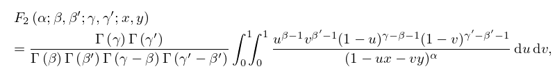
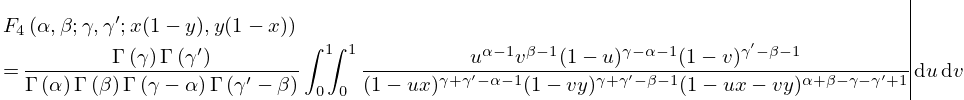
18: 16.15 Integral Representations and Integrals

… ►

16.15.1 $$F_1(\alpha ;\beta ,{\beta }^{\prime };\gamma ;x,y)=\frac{\mathrm{\Gamma }\left(\gamma \right)}{\mathrm{\Gamma }\left(\alpha \right)\mathrm{\Gamma }\left(\gamma -\alpha \right)}{\int }_0^1\frac{u^{\alpha -1}{(1-u)}^{\gamma -\alpha -1}}{{(1-ux)}^{\beta }{(1-uy)}^{{\beta }^{\prime }}}du,$$ $\mathrm{\Re }\alpha >0$, $\mathrm{\Re }\left(\gamma -\alpha \right)>0$,

ⓘ

Symbols:

$F_1(\alpha ;\beta ,{\beta }^{\prime };\gamma ;x,y)$: first Appell function, $\mathrm{\Gamma }\left(z\right)$: gamma function, $dx$: differential of $x$ , $\int$: integral and $\mathrm{\Re }$: real part

Keywords:

Mellin transform

Permalink:

http://dlmf.nist.gov/16.15.E1

Encodings:

pMML, png, TeX

See also:

Annotations for §16.15 and Ch.16

►

16.15.2 $$F_2(\alpha ;\beta ,{\beta }^{\prime };\gamma ,{\gamma }^{\prime };x,y)=\frac{\mathrm{\Gamma }\left(\gamma \right)\mathrm{\Gamma }\left({\gamma }^{\prime }\right)}{\mathrm{\Gamma }\left(\beta \right)\mathrm{\Gamma }\left({\beta }^{\prime }\right)\mathrm{\Gamma }\left(\gamma -\beta \right)\mathrm{\Gamma }\left({\gamma }^{\prime }-{\beta }^{\prime }\right)}{\int }_0^1{\int }_0^1\frac{u^{\beta -1}{v}^{{\beta }^{\prime }-1}{(1-u)}^{\gamma -\beta -1}{(1-v)}^{{\gamma }^{\prime }-{\beta }^{\prime }-1}}{{(1-ux-vy)}^{\alpha }}dudv,$$ $\mathrm{\Re }\gamma >\mathrm{\Re }\beta >0$, $\mathrm{\Re }{\gamma }^{\prime }>\mathrm{\Re }{\beta }^{\prime }>0$,

ⓘ

Symbols:

$F_2(\alpha ;\beta ,{\beta }^{\prime };\gamma ,{\gamma }^{\prime };x,y)$: second Appell function, $\mathrm{\Gamma }\left(z\right)$: gamma function, $dx$: differential of $x$ , $\int$: integral and $\mathrm{\Re }$: real part

Keywords:

Mellin transform

Permalink:

http://dlmf.nist.gov/16.15.E2

Encodings:

pMML, png, TeX

See also:

Annotations for §16.15 and Ch.16

►

16.15.3 $$F_3(\alpha ,{\alpha }^{\prime };\beta ,{\beta }^{\prime };\gamma ;x,y)=\frac{\mathrm{\Gamma }\left(\gamma \right)}{\mathrm{\Gamma }\left(\beta \right)\mathrm{\Gamma }\left({\beta }^{\prime }\right)\mathrm{\Gamma }\left(\gamma -\beta -{\beta }^{\prime }\right)}{\iint }_{\mathrm{\Delta }}\frac{u^{\beta -1}{v}^{{\beta }^{\prime }-1}{(1-u-v)}^{\gamma -\beta -{\beta }^{\prime }-1}}{{(1-ux)}^{\alpha }{(1-vy)}^{{\alpha }^{\prime }}}dudv,$$ $\mathrm{\Re }\left(\gamma -\beta -{\beta }^{\prime }\right)>0$, $\mathrm{\Re }\beta >0$, $\mathrm{\Re }{\beta }^{\prime }>0$,

ⓘ

Symbols:

$F_3(\alpha ,{\alpha }^{\prime };\beta ,{\beta }^{\prime };\gamma ;x,y)$: third Appell function, $\mathrm{\Gamma }\left(z\right)$: gamma function, $dx$: differential of $x$ and $\mathrm{\Re }$: real part

Keywords:

Mellin transform

Notes:

Erdélyi et al. (1953a, 5.8.1(3)) contains a typo.

Referenced by:

Erratum (V1.0.14) for Equation (16.15.3), Erratum (V1.0.14) for Equation (16.15.3)

Permalink:

http://dlmf.nist.gov/16.15.E3

Encodings:

pMML, png, TeX

Clarification (effective with 1.0.14):

A stray “$f$” was removed; it appeared after the comma at the end of this equation.

See also:

Annotations for §16.15 and Ch.16

… ►

16.15.4 $$F_4(\alpha ,\beta ;\gamma ,{\gamma }^{\prime };x(1-y),y(1-x))=\frac{\mathrm{\Gamma }\left(\gamma \right)\mathrm{\Gamma }\left({\gamma }^{\prime }\right)}{\mathrm{\Gamma }\left(\alpha \right)\mathrm{\Gamma }\left(\beta \right)\mathrm{\Gamma }\left(\gamma -\alpha \right)\mathrm{\Gamma }\left({\gamma }^{\prime }-\beta \right)}{\int }_0^1{\int }_0^1\frac{u^{\alpha -1}{v}^{\beta -1}{(1-u)}^{\gamma -\alpha -1}{(1-v)}^{{\gamma }^{\prime }-\beta -1}}{{(1-ux)}^{\gamma +{\gamma }^{\prime }-\alpha -1}{(1-vy)}^{\gamma +{\gamma }^{\prime }-\beta -1}{(1-ux-vy)}^{\alpha +\beta -\gamma -{\gamma }^{\prime }+1}}dudv,$$ $\mathrm{\Re }\gamma >\mathrm{\Re }\alpha >0$, $\mathrm{\Re }{\gamma }^{\prime }>\mathrm{\Re }\beta >0$.

ⓘ

Symbols:

$F_4(\alpha ,\beta ;\gamma ,{\gamma }^{\prime };x,y)$: fourth Appell function, $\mathrm{\Gamma }\left(z\right)$: gamma function, $dx$: differential of $x$ , $\int$: integral and $\mathrm{\Re }$: real part

Keywords:

Mellin transform

Source:

Burchnall and Chaundy (1940, (68))

Referenced by:

§16.15

Permalink:

http://dlmf.nist.gov/16.15.E4

Encodings:

pMML, png, TeX

See also:

Annotations for §16.15 and Ch.16

…

19: Bibliography K

… ►

Bernstein, Pick, Poisson and related integral expressions for Lambert $W$ . Integral Transforms Spec. Funct. 23 (11), pp. 817–829.

ⓘ

External Links:

ISSN 1065-2469, Document, Link, MathReview (Ross C. McPhedran), ZentralBlatt

Referenced by:

§4.13.

Encodings:

BibTeX

… ►

Tables of the Incomplete Gamma Function Ratio: The Chi-square Integral, the Poisson Distribution. Justus von Liebig Verlag, Darmstadt (German, English).

ⓘ

Notes:

In cooperation with W. Rudert

External Links:

MathReview, ZentralBlatt

Referenced by:

1st item.

Encodings:

BibTeX

… ►

Computation of tangent, Euler, and Bernoulli numbers. Math. Comp. 21 (100), pp. 663–688.

ⓘ

External Links:

FullText, MathReview, ZentralBlatt

Referenced by:

§24.15(ii), §24.19(i).

Encodings:

BibTeX

… ►

Asymptotic solution of Maxwell’s equations near caustics. Izv. Vuz. Radiofiz. 7, pp. 1049–1056.

ⓘ

Referenced by:

§36.14(i).

Encodings:

BibTeX

… ►

The Korteweg-de Vries Equation and Related Evolution Equations. In Nonlinear Wave Motion (Proc. AMS-SIAM Summer Sem., Clarkson Coll. Tech., Potsdam, N.Y., 1972), A. C. Newell (Ed.), Lectures in Appl. Math., Vol. 15, pp. 61–83.

ⓘ

External Links:

MathReview (G. L. Lamb, Jr.), ZentralBlatt

Referenced by:

§22.19(iii).

Encodings:

BibTeX

…

20: 30.1 Special Notation

… ► ►►►

$x$	real variable. Except in §§30.7(iv), 30.11(ii), 30.13, and 30.14, .
${\gamma }^2$	real parameter (positive, zero, or negative).
…

►The main functions treated in this chapter are the eigenvalues ${\lambda }_n^m\left({\gamma }^2\right)$ and the spheroidal wave functions ${\mathrm{𝖯𝗌}}_n^m(x,{\gamma }^2)$, ${\mathrm{𝖰𝗌}}_n^m(x,{\gamma }^2)$, ${\mathrm{𝑃𝑠}}_n^m(z,{\gamma }^2)$, ${\mathrm{𝑄𝑠}}_n^m(z,{\gamma }^2)$, and $S_n^{m(j)}(z,\gamma )$, $j=1,2,3,4$. …Meixner and Schäfke (1954) use $\mathrm{ps}$, $\mathrm{qs}$, $\mathrm{Ps}$, $\mathrm{Qs}$ for $\mathrm{𝖯𝗌}$, $\mathrm{𝖰𝗌}$, $\mathrm{𝑃𝑠}$, $\mathrm{𝑄𝑠}$, respectively. … ►Flammer (1957) and Abramowitz and Stegun (1964) use ${\lambda }_{mn}(\gamma )$ for ${\lambda }_n^m\left({\gamma }^2\right)+{\gamma }^2$, $R_{mn}^{(j)}(\gamma ,z)$ for $S_n^{m(j)}(z,\gamma )$, and …where $d_{mn}(\gamma )$ is a normalization constant determined by …