Euler%E2%80%93Maclaurin%20formula
(0.003 seconds)
21—30 of 562 matching pages
21: 15.11 Riemann’s Differential Equation
…
►The most general form is given by
…
►Here , , are the exponent pairs at the points , , , respectively.
…Also, if any of , , , is at infinity, then we take the corresponding limit in (15.11.1).
…
►
§15.11(ii) Transformation Formulas
… ►These constants can be chosen to map any two sets of three distinct points and onto each other. …22: Bibliography K
…
►
A proof of the -Macdonald-Morris conjecture for
.
Mem. Amer. Math. Soc. 108 (516), pp. vi+80.
…
►
Linear convergence and the bisection algorithm.
Amer. Math. Monthly 93 (1), pp. 48–51.
…
►
On formulas involving both the Bernoulli and Fibonacci numbers.
Scripta Math. 23, pp. 27–35.
…
►
Connection formulae for asymptotics of solutions of the degenerate third Painlevé equation. I.
Inverse Problems 20 (4), pp. 1165–1206.
…
►
Computation of tangent, Euler, and Bernoulli numbers.
Math. Comp. 21 (100), pp. 663–688.
…
23: 15.10 Hypergeometric Differential Equation
…
►
§15.10(ii) Kummer’s 24 Solutions and Connection Formulas
… ►The connection formulas for the principal branches of Kummer’s solutions are: ►
15.10.17
…
►
15.10.21
…
►
15.10.25
…
24: 25.2 Definition and Expansions
…
►where the Stieltjes constants are defined via
…
►
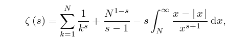
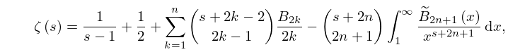
§25.2(iii) Representations by the Euler–Maclaurin Formula
►
25.2.8
, .
…
►
25.2.10
, .
…
►product over zeros of with (see §25.10(i)); is Euler’s constant (§5.2(ii)).
25: 30.9 Asymptotic Approximations and Expansions
…
►
§30.9(i) Prolate Spheroidal Wave Functions
►As , with , … ►The asymptotic behavior of and as in descending powers of is derived in Meixner (1944). …The asymptotic behavior of and as is given in Erdélyi et al. (1955, p. 151). The behavior of for complex and large is investigated in Hunter and Guerrieri (1982). …26: 24.18 Physical Applications
§24.18 Physical Applications
►Bernoulli polynomials appear in statistical physics (Ordóñez and Driebe (1996)), in discussions of Casimir forces (Li et al. (1991)), and in a study of quark-gluon plasma (Meisinger et al. (2002)). ►Euler polynomials also appear in statistical physics as well as in semi-classical approximations to quantum probability distributions (Ballentine and McRae (1998)).27: 32.8 Rational Solutions
…
►In the general case assume , so that as in §32.2(ii) we may set and .
…
►
(a)
…
►
(c)
►
(d)
►
(e)
…
and , where , is odd, and when .
, , and , with even.
, , and , with even.
, , and .
28: 5.5 Functional Relations
…
►
§5.5(ii) Reflection
… ►§5.5(iii) Multiplication
►Duplication Formula
… ►Gauss’s Multiplication Formula
… ►If a positive function on satisfies , , and is convex (see §1.4(viii)), then .29: 24.20 Tables
§24.20 Tables
… ►Wagstaff (1978) gives complete prime factorizations of and for and , respectively. …30: 12.12 Integrals
…
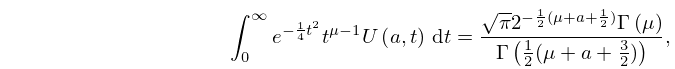
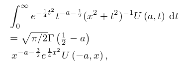
►
12.12.1
,
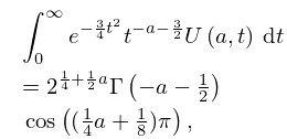
►
12.12.2
,
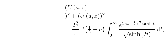
►
12.12.3
.
…
►
12.12.4
.
…
►For compendia of integrals see Erdélyi et al. (1953b, v. 2, pp. 121–122), Erdélyi et al. (1954a, b, v. 1, pp. 60–61, 115, 210–211, and 336;
v. 2, pp. 76–80, 115, 151, 171, and 395–398), Gradshteyn and Ryzhik (2000, §7.7), Magnus et al. (1966, pp. 330–331), Marichev (1983, pp. 190–191), Oberhettinger (1974, pp. 144–145), Oberhettinger (1990, pp. 106–108 and 192), Oberhettinger and Badii (1973, pp. 181–185), Prudnikov et al. (1986b, pp. 36–37, 155–168, 243–246, 289–290, 327–328, 419–420, and 619), Prudnikov et al. (1992a, §3.11), and Prudnikov et al. (1992b, §3.11).
…
