Cauchy determinant

SearchAdvancedHelp

(0.001 seconds)

11—20 of 68 matching pages

11: 32.10 Special Function Solutions

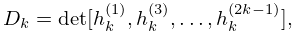
… ►where ${\tau }_n(z)$ is the $n\times n$ Wronskian determinant … ►For determinantal representations see Forrester and Witte (2002) and Okamoto (1987c). … ►For determinantal representations see Forrester and Witte (2001) and Okamoto (1986). … ►For determinantal representations see Forrester and Witte (2002), Masuda (2004), and Okamoto (1987b). … ►For determinantal representations see Forrester and Witte (2004) and Masuda (2004). …

12: 1.11 Zeros of Polynomials

… ►

►

… ►

1.11.26 $$D_k=det[h_k^{(1)},h_k^{(3)},\mathrm{\dots },h_k^{(2k-1)}],$$

ⓘ

Symbols:

$det$: determinant, $k$: integer and $D_j$: quantities

Permalink:

http://dlmf.nist.gov/1.11.E26

Encodings:

pMML, png, TeX

See also:

Annotations for §1.11(v), §1.11(v), §1.11 and Ch.1

…

13: 4.10 Integrals

… ►

4.10.7 $${⨍}_0^x\frac{dt}{\ln t}=\mathrm{li}\left(x\right),$$ $x>1$.

ⓘ

Symbols:

$dx$: differential of $x$ , $\mathrm{li}\left(x\right)$: logarithmic integral, $\ln z$: principal branch of logarithm function, ${⨍}_a^b$: Cauchy principal value and $x$: real variable

A&S Ref:

4.1.57

Referenced by:

§4.10(i)

Permalink:

http://dlmf.nist.gov/4.10.E7

Encodings:

pMML, png, TeX

See also:

Annotations for §4.10(i), §4.10 and Ch.4

►The left-hand side of (4.10.7) is a Cauchy principal value (§1.4(v)). …

14: 35.1 Special Notation

… ► ►►►

$a,b$	complex variables.
…
$\left|𝐗\right|$	determinant of $𝐗$ (except when $m=1$ where it means either determinant or absolute value, depending on the context).
…

…

15: 35.3 Multivariate Gamma and Beta Functions

… ►

35.3.1 $${\mathrm{\Gamma }}_m\left(a\right)={\int }_{𝛀}\mathrm{etr}\left(-𝐗\right){\left|𝐗\right|}^{a-\frac{1}{2}(m+1)}d𝐗,$$ $\mathrm{\Re }\left(a\right)>\frac{1}{2}(m-1)$.

ⓘ

Symbols:

$\mathrm{etr}\left(𝐀\right)$: exponential of trace, $\int$: integral, ${\mathrm{\Gamma }}_m\left(a\right)$: multivariate gamma function, $\mathrm{\Re }$: real part, $a$: complex variable, $𝐗$: real symmetric $m\times m$ matrix, $\left|𝐗\right|$: determinant of $𝐗$ , $d$: differential of matrix, $𝛀$: space of positive-definite real symmetric $m\times m$ matrices and $m$: positive integer

Permalink:

http://dlmf.nist.gov/35.3.E1

Encodings:

pMML, png, TeX

See also:

Annotations for §35.3(i), §35.3 and Ch.35

►

35.3.2 $${\mathrm{\Gamma }}_m\left(s_1,\mathrm{\dots },s_m\right)={\int }_{𝛀}\mathrm{etr}\left(-𝐗\right){\left|𝐗\right|}^{s_m-\frac{1}{2}(m+1)}\prod _{j=1}^{m-1}{|{(𝐗)}_j|}^{s_j-s_{j+1}}d𝐗,$$ $s_j\in ℂ$, $\mathrm{\Re }\left(s_j\right)>\frac{1}{2}(j-1)$, $j=1,\mathrm{\dots },m$.

ⓘ

Symbols:

$ℂ$: complex plane, $\in$: element of, $\mathrm{etr}\left(𝐀\right)$: exponential of trace, $\int$: integral, ${\mathrm{\Gamma }}_m\left(a\right)$: multivariate gamma function, $\mathrm{\Re }$: real part, $𝐗$: real symmetric $m\times m$ matrix, $\left|𝐗\right|$: determinant of $𝐗$ , $|{(𝐗)}_j|$: $j$th principal minor of $𝐗$ , $d$: differential of matrix, $𝛀$: space of positive-definite real symmetric $m\times m$ matrices, $j$: nonnegative integer and $m$: positive integer

Permalink:

http://dlmf.nist.gov/35.3.E2

Encodings:

pMML, png, TeX

See also:

Annotations for §35.3(i), §35.3 and Ch.35

►

35.3.3 $\mathrm{\Re }\left(a\right),\mathrm{\Re }\left(b\right)>\frac{1}{2}(m-1)$.

ⓘ

Defines:

${\mathrm{B}}_m(a,b)$: multivariate beta function

Symbols:

$\int$: integral, $\mathrm{\Re }$: real part, $a$: complex variable, $𝐈$: $m\times m$ identity matrix, $𝐗$: real symmetric $m\times m$ matrix, $\left|𝐗\right|$: determinant of $𝐗$ , $d$: differential of matrix, $b$: complex variable, : less-than for matrices, $m$: positive integer and $𝟎$: $m\times m$ matrix of zeros

Keywords:

definition, multivariate beta function

Permalink:

http://dlmf.nist.gov/35.3.E3

Encodings:

pMML, png, TeX

See also:

Annotations for §35.3(i), §35.3 and Ch.35

… ►

35.3.8 $${\mathrm{B}}_m(a,b)={\int }_{𝛀}{\left|𝐗\right|}^{a-\frac{1}{2}(m+1)}{\left|𝐈+𝐗\right|}^{-(a+b)}d𝐗,$$ $\mathrm{\Re }\left(a\right),\mathrm{\Re }\left(b\right)>\frac{1}{2}(m-1)$.

ⓘ

Symbols:

$\int$: integral, ${\mathrm{B}}_m(a,b)$: multivariate beta function, $\mathrm{\Re }$: real part, $a$: complex variable, $𝐈$: $m\times m$ identity matrix, $𝐗$: real symmetric $m\times m$ matrix, $\left|𝐗\right|$: determinant of $𝐗$ , $d$: differential of matrix, $𝛀$: space of positive-definite real symmetric $m\times m$ matrices, $b$: complex variable and $m$: positive integer

Permalink:

http://dlmf.nist.gov/35.3.E8

Encodings:

pMML, png, TeX

See also:

Annotations for §35.3(ii), §35.3 and Ch.35

16: 22.8 Addition Theorems

… ►

22.8.20

ⓘ

Symbols:

$\mathrm{cn}(z,k)$: Jacobian elliptic function, $\mathrm{dn}(z,k)$: Jacobian elliptic function, $\mathrm{sn}(z,k)$: Jacobian elliptic function, $det$: determinant, $z$: complex and $k$: modulus

Referenced by:

§22.8(iii)

Permalink:

http://dlmf.nist.gov/22.8.E20

Encodings:

pMML, png, TeX

See also:

Annotations for §22.8(iii), §22.8 and Ch.22

… ►

22.8.23

ⓘ

Symbols:

$\mathrm{cn}(z,k)$: Jacobian elliptic function, $\mathrm{dn}(z,k)$: Jacobian elliptic function, $\mathrm{sn}(z,k)$: Jacobian elliptic function, $det$: determinant, $z$: complex and $k$: modulus

Permalink:

http://dlmf.nist.gov/22.8.E23

Encodings:

pMML, png, TeX

See also:

Annotations for §22.8(iii), §22.8 and Ch.22

…

17: 19.3 Graphics

… ►

►►

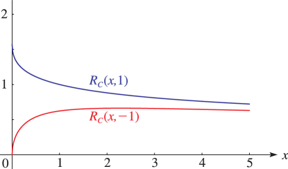
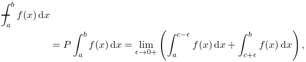
Figure 19.3.2: $R_C(x,1)$ and the Cauchy principal value of $R_C(x,-1)$ for $0\le x\le 5$. … Magnify

… ►

►

►

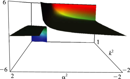
Figure 19.3.5: $\mathrm{\Pi }({\alpha }^2,k)$ as a function of $k^2$ and ${\alpha }^2$ for , $-2\le {\alpha }^2\le 2$. Cauchy principal values are shown when ${\alpha }^2>1$. … Magnify 3D Help

►

►

►

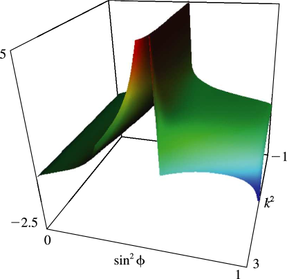
Figure 19.3.6: $\mathrm{\Pi }(\varphi ,2,k)$ as a function of $k^2$ and ${\sin }^2\varphi$ for $-1\le k^2\le 3$, . Cauchy principal values are shown when ${\sin }^2\varphi >\frac{1}{2}$. …If ${\sin }^2\varphi =1$ ($>k^2$), then the function reduces to $\mathrm{\Pi }(2,k)$ with Cauchy principal value $K\left(k\right)-\mathrm{\Pi }(\frac{1}{2}{k}^2,k)$, which tends to $-\mathrm{\infty }$ as $k^2\to 1-$. …If ${\sin }^2\varphi =1/k^2$ (), then by (19.7.4) it reduces to $\mathrm{\Pi }(2/k^2,1/k)/k$, $k^2\ne 2$, with Cauchy principal value $(K\left(1/k\right)-\mathrm{\Pi }(\frac{1}{2},1/k))/k$, , by (19.6.5). … Magnify 3D Help

…

18: 35.5 Bessel Functions of Matrix Argument

… ►

35.5.3 $$B_{\nu }\left(𝐓\right)={\int }_{𝛀}\mathrm{etr}\left(-(𝐓𝐗+{𝐗}^{-1})\right){\left|𝐗\right|}^{\nu -\frac{1}{2}(m+1)}d𝐗,$$ $\nu \in ℂ$, $𝐓\in 𝛀$.

ⓘ

Defines:

$B_{\nu }\left(𝐓\right)$: Bessel function of matrix argument (second kind)

Symbols:

$ℂ$: complex plane, $\in$: element of, $\mathrm{etr}\left(𝐀\right)$: exponential of trace, $\int$: integral, $𝐓$: real symmetric $m\times m$ matrix, $𝐗$: real symmetric $m\times m$ matrix, $\left|𝐗\right|$: determinant of $𝐗$ , $d$: differential of matrix, $𝛀$: space of positive-definite real symmetric $m\times m$ matrices and $m$: positive integer

Referenced by:

§35.9

Permalink:

http://dlmf.nist.gov/35.5.E3

Encodings:

pMML, png, TeX

See also:

Annotations for §35.5(i), §35.5 and Ch.35

… ►

35.5.4 $${\int }_{𝛀}\mathrm{etr}\left(-𝐓𝐗\right){\left|𝐗\right|}^{\nu }{A}_{\nu }\left(𝐒𝐗\right)d𝐗=\mathrm{etr}\left(-𝐒{𝐓}^{-1}\right){\left|𝐓\right|}^{-\nu -\frac{1}{2}(m+1)},$$ $𝐒\in 𝓢$, $𝐓\in 𝛀$; $\mathrm{\Re }\left(\nu \right)>-1$.

ⓘ

Symbols:

$A_{\nu }\left(𝐓\right)$: Bessel function of matrix argument (first kind), $\in$: element of, $\mathrm{etr}\left(𝐀\right)$: exponential of trace, $\int$: integral, $\mathrm{\Re }$: real part, $𝓢$: space of real symmetric $m\times m$ matrices, $𝐒$: real symmetric $m\times m$ matrix, $𝐓$: real symmetric $m\times m$ matrix, $𝐗$: real symmetric $m\times m$ matrix, $\left|𝐗\right|$: determinant of $𝐗$ , $d$: differential of matrix, $𝛀$: space of positive-definite real symmetric $m\times m$ matrices and $m$: positive integer

Permalink:

http://dlmf.nist.gov/35.5.E4

Encodings:

pMML, png, TeX

See also:

Annotations for §35.5(ii), §35.5 and Ch.35

►

35.5.5 ${\nu }_j\in ℂ$, $\mathrm{\Re }\left({\nu }_j\right)>-1$, $j=1,2$; ${𝐒}_1,{𝐒}_2\in 𝓢$; $𝐓\in 𝛀$.

ⓘ

Symbols:

$A_{\nu }\left(𝐓\right)$: Bessel function of matrix argument (first kind), $ℂ$: complex plane, $\in$: element of, $\int$: integral, $\mathrm{\Re }$: real part, $𝓢$: space of real symmetric $m\times m$ matrices, $𝐒$: real symmetric $m\times m$ matrix, $𝐓$: real symmetric $m\times m$ matrix, $𝐗$: real symmetric $m\times m$ matrix, $\left|𝐗\right|$: determinant of $𝐗$ , $d$: differential of matrix, $𝛀$: space of positive-definite real symmetric $m\times m$ matrices, : less-than for matrices, $j$: nonnegative integer, $m$: positive integer and $𝟎$: $m\times m$ matrix of zeros

Permalink:

http://dlmf.nist.gov/35.5.E5

Encodings:

pMML, png, TeX

See also:

Annotations for §35.5(ii), §35.5 and Ch.35

►

35.5.6 $$B_{\nu }\left(𝐓\right)={\left|𝐓\right|}^{-\nu }{B}_{-\nu }\left(𝐓\right),$$ $\nu \in ℂ$, $𝐓\in 𝛀$.

ⓘ

Symbols:

$B_{\nu }\left(𝐓\right)$: Bessel function of matrix argument (second kind), $ℂ$: complex plane, $\in$: element of, $𝐓$: real symmetric $m\times m$ matrix, $\left|𝐗\right|$: determinant of $𝐗$ and $𝛀$: space of positive-definite real symmetric $m\times m$ matrices

Permalink:

http://dlmf.nist.gov/35.5.E6

Encodings:

pMML, png, TeX

See also:

Annotations for §35.5(ii), §35.5 and Ch.35

►

35.5.7 $${\int }_{𝛀}{A}_{{\nu }_1}\left(𝐓𝐗\right)B_{-{\nu }_2}\left(𝐒𝐗\right){\left|𝐗\right|}^{{\nu }_1}d𝐗=\frac{1}{A_{{\nu }_1+{\nu }_2}\left(𝟎\right)}{\left|𝐒\right|}^{{\nu }_2}{\left|𝐓+𝐒\right|}^{-({\nu }_1+{\nu }_2+\frac{1}{2}(m+1))},$$ $\mathrm{\Re }\left({\nu }_1+{\nu }_2\right)>-1$; $𝐒,𝐓\in 𝛀$.

ⓘ

Symbols:

$A_{\nu }\left(𝐓\right)$: Bessel function of matrix argument (first kind), $B_{\nu }\left(𝐓\right)$: Bessel function of matrix argument (second kind), $\in$: element of, $\int$: integral, $\mathrm{\Re }$: real part, $𝐒$: real symmetric $m\times m$ matrix, $𝐓$: real symmetric $m\times m$ matrix, $𝐗$: real symmetric $m\times m$ matrix, $\left|𝐗\right|$: determinant of $𝐗$ , $d$: differential of matrix, $𝛀$: space of positive-definite real symmetric $m\times m$ matrices, $m$: positive integer and $𝟎$: $m\times m$ matrix of zeros

Permalink:

http://dlmf.nist.gov/35.5.E7

Encodings:

pMML, png, TeX

See also:

Annotations for §35.5(ii), §35.5 and Ch.35

…

19: 1.9 Calculus of a Complex Variable

… ►

Cauchy–Riemann Equations

… ►

Cauchy’s Theorem

… ►

Cauchy’s Integral Formula

…

20: 1.4 Calculus of One Variable

… ►

Cauchy Principal Values

… ►

1.4.24 $${⨍}_a^{b}f(x)dx=𝑃{\int }_a^{b}f(x)dx=\underset{ϵ\to 0+}{lim}\left({\int }_a^{c-ϵ}f(x)dx+{\int }_{c+ϵ}^{b}f(x)dx\right),$$

ⓘ

Defines:

${⨍}_a^b$: Cauchy principal value

Symbols:

$dx$: differential of $x$ and $\int$: integral

Referenced by:

§1.18(vi)

Permalink:

http://dlmf.nist.gov/1.4.E24

Encodings:

pMML, png, TeX

See also:

Annotations for §1.4(v), §1.4(v), §1.4 and Ch.1

… ►

1.4.25 $${⨍}_{-\mathrm{\infty }}^{\mathrm{\infty }}f(x)dx=𝑃{\int }_{-\mathrm{\infty }}^{\mathrm{\infty }}f(x)dx=\underset{b\to \mathrm{\infty }}{lim}{\int }_{-b}^{b}f(x)dx,$$

ⓘ

Symbols:

$dx$: differential of $x$ , $\int$: integral and ${⨍}_a^b$: Cauchy principal value

Referenced by:

§1.14(i)

Permalink:

http://dlmf.nist.gov/1.4.E25

Encodings:

pMML, png, TeX

See also:

Annotations for §1.4(v), §1.4(v), §1.4 and Ch.1

…