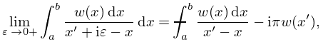
Cauchy–Schwarz inequalities for sums and integrals

SearchAdvancedHelp

(0.002 seconds)

21—30 of 196 matching pages

21: 19.7 Connection Formulas

… ►The first of the three relations maps each circular region onto itself and each hyperbolic region onto the other; in particular, it gives the Cauchy principal value of $\mathrm{\Pi }(\varphi ,{\alpha }^2,k)$ when ${\alpha }^2>{\csc }^2\varphi$ (see (19.6.5) for the complete case). …

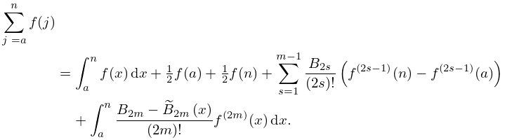
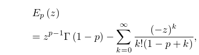
22: 2.10 Sums and Sequences

… ►

2.10.1 $$\sum _{j=a}^{n}f(j)={\int }_a^{n}f(x)dx+\frac{1}{2}f(a)+\frac{1}{2}f(n)+\sum _{s=1}^{m-1}\frac{B_{2s}}{(2s)!}\left(f^{(2s-1)}(n)-f^{(2s-1)}(a)\right)+{\int }_a^n\frac{B_{2m}-{\tilde{B}}_{2m}\left(x\right)}{(2m)!}{f}^{(2m)}(x)dx.$$

ⓘ

Symbols:

$B_n$: Bernoulli numbers, $dx$: differential of $x$ , $!$: factorial (as in $n!$), $\int$: integral, ${\tilde{B}}_n\left(x\right)$: periodic Bernoulli functions, $a$: integer, $m$: integer, $n$: integer and $f(x)$: integrable function

Referenced by:

§2.10(i), §2.10(i)

Permalink:

http://dlmf.nist.gov/2.10.E1

Encodings:

pMML, png, TeX

See also:

Annotations for §2.10(i), §2.10 and Ch.2

… ►

The first infinite integral in (2.10.2) converges.

… ►For an extension to integrals with Cauchy principal values see Elliott (1998). … ►The asymptotic behavior of entire functions defined by Maclaurin series can be approached by converting the sum into a contour integral by use of the residue theorem and applying the methods of §§2.4 and 2.5. … ►These problems can be brought within the scope of §2.4 by means of Cauchy’s integral formula …

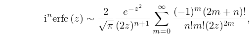
23: 7.18 Repeated Integrals of the Complementary Error Function

… ►

7.18.6 $${\mathrm{i}}^n\mathrm{erfc}\left(z\right)=\sum _{k=0}^{\mathrm{\infty }}\frac{{(-1)}^k{z}^k}{2^{n-k}k!\mathrm{\Gamma }\left(1+\frac{1}{2}(n-k)\right)}.$$

ⓘ

Symbols:

$\mathrm{\Gamma }\left(z\right)$: gamma function, $!$: factorial (as in $n!$), ${\mathrm{i}}^n\mathrm{erfc}\left(z\right)$: repeated integrals of the complementary error function, $z$: complex variable and $n$: nonnegative integer

A&S Ref:

7.2.4

Permalink:

http://dlmf.nist.gov/7.18.E6

Encodings:

pMML, png, TeX

See also:

Annotations for §7.18(iii), §7.18 and Ch.7

… ►

7.18.14 $${\mathrm{i}}^n\mathrm{erfc}\left(z\right)\sim \frac{2}{\sqrt{\pi }}\frac{{\mathrm{e}}^{-z^2}}{{(2z)}^{n+1}}\sum _{m=0}^{\mathrm{\infty }}\frac{{(-1)}^m(2m+n)!}{n!m!{(2z)}^{2m}},$$ $z\to \mathrm{\infty }$, .

ⓘ

Symbols:

$\sim$: Poincaré asymptotic expansion, $\pi$: the ratio of the circumference of a circle to its diameter, $\mathrm{e}$: base of natural logarithm, $!$: factorial (as in $n!$), $\mathrm{ph}$: phase, ${\mathrm{i}}^n\mathrm{erfc}\left(z\right)$: repeated integrals of the complementary error function, $z$: complex variable and $n$: nonnegative integer

A&S Ref:

7.2.14

Permalink:

http://dlmf.nist.gov/7.18.E14

Encodings:

pMML, png, TeX

See also:

Annotations for §7.18(vi), §7.18 and Ch.7

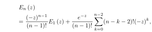
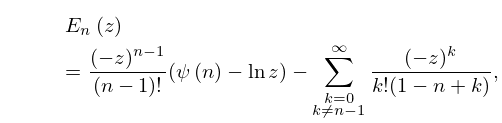
24: 8.19 Generalized Exponential Integral

… ►

8.19.7 $$E_n\left(z\right)=\frac{{(-z)}^{n-1}}{(n-1)!}{E}_1\left(z\right)+\frac{{\mathrm{e}}^{-z}}{(n-1)!}\sum _{k=0}^{n-2}(n-k-2)!{(-z)}^k,$$ $n=2,3,\mathrm{\dots }$.

ⓘ

Symbols:

$\mathrm{e}$: base of natural logarithm, $E_1\left(z\right)$: exponential integral, $E_p\left(z\right)$: generalized exponential integral, $!$: factorial (as in $n!$), $z$: complex variable, $k$: nonnegative integer and $n$: nonnegative integer

Permalink:

http://dlmf.nist.gov/8.19.E7

Encodings:

pMML, png, TeX

See also:

Annotations for §8.19(iii), §8.19 and Ch.8

… ►

8.19.8 $$E_n\left(z\right)=\frac{{(-z)}^{n-1}}{(n-1)!}(\psi \left(n\right)-\ln z)-\sum _{\begin{array}{c}k=0\\ k\ne n-1\end{array}}^{\mathrm{\infty }}\frac{{(-z)}^k}{k!(1-n+k)},$$

ⓘ

Symbols:

$\psi \left(z\right)$: psi (or digamma) function, $E_p\left(z\right)$: generalized exponential integral, $!$: factorial (as in $n!$), $\ln z$: principal branch of logarithm function, $z$: complex variable, $k$: nonnegative integer and $n$: nonnegative integer

A&S Ref:

5.1.12

Referenced by:

§8.19(iv)

Permalink:

http://dlmf.nist.gov/8.19.E8

Encodings:

pMML, png, TeX

See also:

Annotations for §8.19(iv), §8.19 and Ch.8

… ►

8.19.10 $$E_p\left(z\right)=z^{p-1}\mathrm{\Gamma }\left(1-p\right)-\sum _{k=0}^{\mathrm{\infty }}\frac{{(-z)}^k}{k!(1-p+k)},$$

ⓘ

Symbols:

$\mathrm{\Gamma }\left(z\right)$: gamma function, $E_p\left(z\right)$: generalized exponential integral, $!$: factorial (as in $n!$), $z$: complex variable, $p$: parameter and $k$: nonnegative integer

Referenced by:

§8.19(iv)

Permalink:

http://dlmf.nist.gov/8.19.E10

Encodings:

pMML, png, TeX

See also:

Annotations for §8.19(iv), §8.19 and Ch.8

… ►

§8.19(ix) Inequalities

… ►

8.19.24 $${\int }_0^{\mathrm{\infty }}{\mathrm{e}}^{-at}{E}_n\left(t\right)dt=\frac{{(-1)}^{n-1}}{a^n}\left(\ln \left(1+a\right)+\sum _{k=1}^{n-1}\frac{{(-1)}^k{a}^k}{k}\right),$$ $n=1,2,\mathrm{\dots }$, $\mathrm{\Re }a>-1$,

ⓘ

Symbols:

$dx$: differential of $x$ , $\mathrm{e}$: base of natural logarithm, $E_p\left(z\right)$: generalized exponential integral, $\int$: integral, $\ln z$: principal branch of logarithm function, $\mathrm{\Re }$: real part, $a$: parameter, $k$: nonnegative integer and $n$: nonnegative integer

A&S Ref:

5.1.34

Referenced by:

§8.19(x)

Permalink:

http://dlmf.nist.gov/8.19.E24

Encodings:

pMML, png, TeX

See also:

Annotations for §8.19(x), §8.19 and Ch.8

…

25: 18.40 Methods of Computation

… ►

18.40.6 $$\underset{\epsilon \to 0+}{lim}{\int }_a^b\frac{w(x)dx}{x^{\prime }+\mathrm{i}\epsilon -x}dx={⨍}_a^b\frac{w(x)dx}{x^{\prime }-x}-\mathrm{i}\pi w(x^{\prime }),$$

ⓘ

Symbols:

$dx$: differential of $x$ , $\mathrm{i}$: imaginary unit, $\int$: integral, ${⨍}_a^b$: Cauchy principal value, $w(x)$: weight function and $x$: real variable

Permalink:

http://dlmf.nist.gov/18.40.E6

Encodings:

pMML, png, TeX

See also:

Annotations for §18.40(ii), §18.40(ii), §18.40 and Ch.18

… ►The bottom and top of the steps at the $x_i$ are lower and upper bounds to ${\int }_a^{x_i}d\mu (x)$ as made explicit via the Chebyshev inequalities discussed by Shohat and Tamarkin (1970, pp. 42–43). …

26: 19.8 Quadratic Transformations

… ►

19.8.6 $$E\left(k\right)=\frac{\pi }{2M(1,k^{\prime })}\left(a_0^2-\sum _{n=0}^{\mathrm{\infty }}{2}^{n-1}{c}_n^2\right)=K\left(k\right)\left(a_1^2-\sum _{n=2}^{\mathrm{\infty }}{2}^{n-1}{c}_n^2\right),$$ , $a_0=1$, $g_0=k^{\prime }$,

ⓘ

Symbols:

$M(a,g)$: arithmetic-geometric mean, $\pi$: the ratio of the circumference of a circle to its diameter, $K\left(k\right)$: Legendre’s complete elliptic integral of the first kind, $E\left(k\right)$: Legendre’s complete elliptic integral of the second kind, $n$: nonnegative integer, $k$: real or complex modulus, $k^{\prime }$: complementary modulus, $a_n$: iterate and $g_n$: iterate

Permalink:

http://dlmf.nist.gov/19.8.E6

Encodings:

pMML, png, TeX

See also:

Annotations for §19.8(i), §19.8 and Ch.19

… ►

19.8.7 $$\mathrm{\Pi }({\alpha }^2,k)=\frac{\pi }{4M(1,k^{\prime })}\left(2+\frac{{\alpha }^2}{1-{\alpha }^2}\sum _{n=0}^{\mathrm{\infty }}{Q}_n\right),$$ , ,

ⓘ

Symbols:

$M(a,g)$: arithmetic-geometric mean, $\pi$: the ratio of the circumference of a circle to its diameter, $\mathrm{\Pi }({\alpha }^2,k)$: Legendre’s complete elliptic integral of the third kind, $n$: nonnegative integer, $k$: real or complex modulus, $k^{\prime }$: complementary modulus, ${\alpha }^2$: real or complex parameter and $Q_n$

Referenced by:

§19.8(i)

Permalink:

http://dlmf.nist.gov/19.8.E7

Encodings:

pMML, png, TeX

See also:

Annotations for §19.8(i), §19.8 and Ch.19

… ►

19.8.9 $$\mathrm{\Pi }({\alpha }^2,k)=\frac{\pi }{4M(1,k^{\prime })}\frac{k^2}{k^2-{\alpha }^2}\sum _{n=0}^{\mathrm{\infty }}{Q}_n,$$ , ,

ⓘ

Symbols:

$M(a,g)$: arithmetic-geometric mean, $\pi$: the ratio of the circumference of a circle to its diameter, $\mathrm{\Pi }({\alpha }^2,k)$: Legendre’s complete elliptic integral of the third kind, $n$: nonnegative integer, $k$: real or complex modulus, $k^{\prime }$: complementary modulus, ${\alpha }^2$: real or complex parameter and $Q_n$

Referenced by:

§19.8(i)

Permalink:

http://dlmf.nist.gov/19.8.E9

Encodings:

pMML, png, TeX

See also:

Annotations for §19.8(i), §19.8 and Ch.19

…

27: 36.10 Differential Equations

… ►

36.10.2 $$\frac{{\partial }^{K+1}{\mathrm{\Psi }}_K\left(𝐱\right)}{{\partial x_1}^{K+1}}+\sum _{m=1}^K{(-\mathrm{i})}^{m-K-2}\left(\frac{m{x}_m}{K+2}\right)\frac{{\partial }^{m-1}{\mathrm{\Psi }}_K\left(𝐱\right)}{{\partial x_1}^{m-1}}=0.$$

ⓘ

Symbols:

${\mathrm{\Psi }}_K\left(𝐱\right)$: canonical integral function, $\mathrm{i}$: imaginary unit, $\frac{\partial f}{\partial x}$: partial derivative of $f$ with respect to $x$ , $\partial x$: partial differential of $x$ , $n$: integer, $K$: codimension and $x_{\mathrm{i}}$: real parameter

Permalink:

http://dlmf.nist.gov/36.10.E2

Encodings:

pMML, png, TeX

See also:

Annotations for §36.10(i), §36.10 and Ch.36

…

28: 9.10 Integrals

… ►

9.10.19 $$\mathrm{Bi}\left(x\right)=\frac{3x^{5/4}{\mathrm{e}}^{(2/3)x^{3/2}}}{2\pi }{⨍}_0^{\mathrm{\infty }}\frac{t^{-3/4}{\mathrm{e}}^{-(2/3)t^{3/2}}\mathrm{Ai}\left(t\right)}{x^{3/2}-t^{3/2}}dt,$$ $x>0$,

ⓘ

Symbols:

$\mathrm{Ai}\left(z\right)$: Airy function, $\mathrm{Bi}\left(z\right)$: Airy function, $\pi$: the ratio of the circumference of a circle to its diameter, $dx$: differential of $x$ , $\mathrm{e}$: base of natural logarithm, ${⨍}_a^b$: Cauchy principal value and $x$: real variable

Proof sketch:

To prove this equation, combine (9.2.10) with (9.10.18).

Referenced by:

§9.5(i), Erratum (V1.0.10) for Equation (9.10.19)

Permalink:

http://dlmf.nist.gov/9.10.E19

Encodings:

pMML, png, TeX

Errata (effective with 1.0.10):

The original and incorrect version,

$$\mathrm{Bi}\left(x\right)=\frac{x^{5/4}{\mathrm{e}}^{(2/3)x^{3/2}}}{2^{5/2}\pi }{⨍}_0^{\mathrm{\infty }}\frac{t^{-1/2}{\mathrm{e}}^{-(2/3)t^{3/2}}\mathrm{Ai}\left(t\right)}{x^{3/2}-t^{3/2}}dt$$

taken from Schulten et al. (1979), has been corrected.

Reported 2015-03-20 by Walter Gautschi

See also:

Annotations for §9.10(vii), §9.10 and Ch.9

►where the last integral is a Cauchy principal value (§1.4(v)). …

29: 19.29 Reduction of General Elliptic Integrals

… ►The only cases that are integrals of the third kind are those in which at least one $m_j$ with $j>h$ is a negative integer and those in which $h=4$ and ${\sum }_{j=1}^n{m}_j$ is a positive integer. … ►

19.29.18 $$b_j^{q}I(q{𝐞}_l)=\sum _{r=0}^q\left(\genfrac{}{}{0.0pt}{}{q}{r}\right)b_l^r{d}_{lj}^{q-r}I(r{𝐞}_j),$$ $j,l=1,2,\mathrm{\dots },n$;

ⓘ

Symbols:

$\left(\genfrac{}{}{0.0pt}{}{m}{n}\right)$: binomial coefficient, $l$: nonnegative integer, $n$: nonnegative integer, $I(𝐦)$: integral and $d_{\alpha \beta }$

Referenced by:

§19.29(ii), §19.34

Permalink:

http://dlmf.nist.gov/19.29.E18

Encodings:

pMML, png, TeX

See also:

Annotations for §19.29(ii), §19.29 and Ch.19

…

30: 16.20 Integrals and Series

§16.20 Integrals and Series

►Integrals of the Meijer $G$-function are given in Apelblat (1983, §19), Erdélyi et al. (1953a, §5.5.2), Erdélyi et al. (1954a, §§6.9 and 7.5), Luke (1969a, §3.6), Luke (1975, §5.6), Mathai (1993, §3.10), and Prudnikov et al. (1990, §2.24). … ►