DLMF: Untitled Document

… ►

34.7.1

\begin{Bmatrix}j_{11}&j_{12}&j_{13}\\ j_{21}&j_{22}&j_{13}\\ j_{31}&j_{31}&0\end{Bmatrix}=\frac{(-1)^{j_{12}+j_{21}+j_{13}+j_{31}}}{((2j_{1% 3}+1)(2j_{31}+1))^{\frac{1}{2}}}\begin{Bmatrix}j_{11}&j_{12}&j_{13}\\ j_{22}&j_{21}&j_{31}\end{Bmatrix}.

ⓘ

Symbols:: $\begin{Bmatrix}\NVar{j_{11}}&\NVar{j_{12}}&\NVar{j_{13}}\\ \NVar{j_{21}}&\NVar{j_{22}}&\NVar{j_{23}}\\ \NVar{j_{31}}&\NVar{j_{32}}&\NVar{j_{33}}\end{Bmatrix}$ : $\mathit{9j}$ symbol, $\begin{Bmatrix}\NVar{j_{1}}&\NVar{j_{2}}&\NVar{j_{3}}\\ \NVar{l_{1}}&\NVar{l_{2}}&\NVar{l_{3}}\end{Bmatrix}$ : $\mathit{6j}$ symbol and $j,j_{r}$ : non-negative integers or non-negative integers plus one half.
Permalink:: http://dlmf.nist.gov/34.7.E1
Encodings:: pMML, png, TeX
See also:: Annotations for §34.7(i), §34.7 and Ch.34

… ►

34.7.2

\sum_{j_{12}\,j_{34}}(2j_{12}+1)(2j_{34}+1)(2j_{13}+1)(2j_{24}+1)\begin{% Bmatrix}j_{1}&j_{2}&j_{12}\\ j_{3}&j_{4}&j_{34}\\ j_{13}&j_{24}&j\end{Bmatrix}\begin{Bmatrix}j_{1}&j_{2}&j_{12}\\ j_{3}&j_{4}&j_{34}\\ j^{\prime}_{13}&j^{\prime}_{24}&j\end{Bmatrix}=\delta_{j_{13},j^{\prime}_{13}}% \delta_{j_{24},j^{\prime}_{24}}.

ⓘ

Symbols:: $\delta_{\NVar{j},\NVar{k}}$ : Kronecker delta, $\begin{Bmatrix}\NVar{j_{11}}&\NVar{j_{12}}&\NVar{j_{13}}\\ \NVar{j_{21}}&\NVar{j_{22}}&\NVar{j_{23}}\\ \NVar{j_{31}}&\NVar{j_{32}}&\NVar{j_{33}}\end{Bmatrix}$ : $\mathit{9j}$ symbol and $j,j_{r}$ : non-negative integers or non-negative integers plus one half.
Permalink:: http://dlmf.nist.gov/34.7.E2
Encodings:: pMML, png, TeX
See also:: Annotations for §34.7(iv), §34.7 and Ch.34

… ►

34.7.3

\sum_{j_{13}\,j_{24}}(-1)^{2j_{2}+j_{24}+j_{23}-j_{34}}(2j_{13}+1)(2j_{24}+1)% \begin{Bmatrix}j_{1}&j_{2}&j_{12}\\ j_{3}&j_{4}&j_{34}\\ j_{13}&j_{24}&j\end{Bmatrix}\begin{Bmatrix}j_{1}&j_{3}&j_{13}\\ j_{4}&j_{2}&j_{24}\\ j_{14}&j_{23}&j\end{Bmatrix}=\begin{Bmatrix}j_{1}&j_{2}&j_{12}\\ j_{4}&j_{3}&j_{34}\\ j_{14}&j_{23}&j\end{Bmatrix}.

ⓘ

Symbols:: $\begin{Bmatrix}\NVar{j_{11}}&\NVar{j_{12}}&\NVar{j_{13}}\\ \NVar{j_{21}}&\NVar{j_{22}}&\NVar{j_{23}}\\ \NVar{j_{31}}&\NVar{j_{32}}&\NVar{j_{33}}\end{Bmatrix}$ : $\mathit{9j}$ symbol and $j,j_{r}$ : non-negative integers or non-negative integers plus one half.
Referenced by:: §34.9
Permalink:: http://dlmf.nist.gov/34.7.E3
Encodings:: pMML, png, TeX
See also:: Annotations for §34.7(vi), §34.7 and Ch.34

… ►

34.7.4

\begin{pmatrix}j_{13}&j_{23}&j_{33}\\ m_{13}&m_{23}&m_{33}\end{pmatrix}\begin{Bmatrix}j_{11}&j_{12}&j_{13}\\ j_{21}&j_{22}&j_{23}\\ j_{31}&j_{32}&j_{33}\end{Bmatrix}=\sum_{m_{r1},m_{r2},r=1,2,3}\begin{pmatrix}j% _{11}&j_{12}&j_{13}\\ m_{11}&m_{12}&m_{13}\end{pmatrix}\begin{pmatrix}j_{21}&j_{22}&j_{23}\\ m_{21}&m_{22}&m_{23}\end{pmatrix}\*\begin{pmatrix}j_{31}&j_{32}&j_{33}\\ m_{31}&m_{32}&m_{33}\end{pmatrix}\begin{pmatrix}j_{11}&j_{21}&j_{31}\\ m_{11}&m_{21}&m_{31}\end{pmatrix}\begin{pmatrix}j_{12}&j_{22}&j_{32}\\ m_{12}&m_{22}&m_{32}\end{pmatrix}.

ⓘ

Symbols:: $\begin{Bmatrix}\NVar{j_{11}}&\NVar{j_{12}}&\NVar{j_{13}}\\ \NVar{j_{21}}&\NVar{j_{22}}&\NVar{j_{23}}\\ \NVar{j_{31}}&\NVar{j_{32}}&\NVar{j_{33}}\end{Bmatrix}$ : $\mathit{9j}$ symbol, $\begin{pmatrix}\NVar{j_{1}}&\NVar{j_{2}}&\NVar{j_{3}}\\ \NVar{m_{1}}&\NVar{m_{2}}&\NVar{m_{3}}\end{pmatrix}$ : $\mathit{3j}$ symbol, $j,j_{r}$ : non-negative integers or non-negative integers plus one half. and $r$ : nonnegative integer
Referenced by:: Erratum (V1.0.10) for Equation (34.7.4)
Permalink:: http://dlmf.nist.gov/34.7.E4
Encodings:: pMML, png, TeX
Errata (effective with 1.0.10):: Originally the third $\mathit{3j}$ symbol in the summation was written incorrectly as $\begin{pmatrix}j_{31}&j_{32}&j_{33}\\ m_{13}&m_{23}&m_{33}\end{pmatrix}.$
Reported 2015-01-19 by Yan-Rui Liu
See also:: Annotations for §34.7(vi), §34.7 and Ch.34

►

34.7.5

\sum_{j^{\prime}}(2j^{\prime}+1)\begin{Bmatrix}j_{11}&j_{12}&j^{\prime}\\ j_{21}&j_{22}&j_{23}\\ j_{31}&j_{32}&j_{33}\end{Bmatrix}\begin{Bmatrix}j_{11}&j_{12}&j^{\prime}\\ j_{23}&j_{33}&j\end{Bmatrix}={(-1)^{2j}}\begin{Bmatrix}j_{21}&j_{22}&j_{23}\\ j_{12}&j&j_{32}\end{Bmatrix}\begin{Bmatrix}j_{31}&j_{32}&j_{33}\\ j&j_{11}&j_{21}\end{Bmatrix}.

ⓘ

Symbols:: $\begin{Bmatrix}\NVar{j_{11}}&\NVar{j_{12}}&\NVar{j_{13}}\\ \NVar{j_{21}}&\NVar{j_{22}}&\NVar{j_{23}}\\ \NVar{j_{31}}&\NVar{j_{32}}&\NVar{j_{33}}\end{Bmatrix}$ : $\mathit{9j}$ symbol, $\begin{Bmatrix}\NVar{j_{1}}&\NVar{j_{2}}&\NVar{j_{3}}\\ \NVar{l_{1}}&\NVar{l_{2}}&\NVar{l_{3}}\end{Bmatrix}$ : $\mathit{6j}$ symbol and $j,j_{r}$ : non-negative integers or non-negative integers plus one half.
Permalink:: http://dlmf.nist.gov/34.7.E5
Encodings:: pMML, png, TeX
See also:: Annotations for §34.7(vi), §34.7 and Ch.34

… ►

A. I. Yablonskiĭ (1959) On rational solutions of the second Painlevé equation. Vesti Akad. Navuk. BSSR Ser. Fiz. Tkh. Nauk. 3, pp. 30–35 (Russian).

ⓘ

Referenced by:: §32.8(ii).
Encodings:: BibTeX

… ►

H. A. Yamani and W. P. Reinhardt (1975)

L

-squared discretizations of the continuum: Radial kinetic energy and the Coulomb Hamiltonian. Phys. Rev. A 11 (4), pp. 1144–1156.

ⓘ

Referenced by:: §18.39(iv), §18.39(iv), §18.39(iv), §18.40(ii).
Encodings:: BibTeX

… ►

A. Yu. Yeremin, I. E. Kaporin, and M. K. Kerimov (1988) Computation of the derivatives of the Riemann zeta-function in the complex domain. USSR Comput. Math. and Math. Phys. 28 (4), pp. 115–124.

ⓘ

Notes:: Includes Fortran programs.
External Links:: Document, ZentralBlatt
Referenced by:: §25.18(i), §25.21(iii).
Encodings:: BibTeX

…

… ►

Table 27.2.1: Primes.

► ►►►

$n$	$p_{n}$	$p_{n+10}$	$p_{n+20}$	$p_{n+30}$	$p_{n+40}$	$p_{n+50}$	$p_{n+60}$	$p_{n+70}$	$p_{n+80}$	$p_{n+90}$
…
5	11	47	97	149	197	257	313	379	439	499
…

► ►

Table 27.2.2: Functions related to division.

► ►►►►►►

$n$	$\phi\left(n\right)$	$d\left(n\right)$	$\sigma\left(n\right)$	$n$	$\phi\left(n\right)$	$d\left(n\right)$	$\sigma\left(n\right)$	$n$	$\phi\left(n\right)$	$d\left(n\right)$	$\sigma\left(n\right)$	$n$	$\phi\left(n\right)$	$d\left(n\right)$	$\sigma\left(n\right)$
…
3	2	2	4	16	8	5	31	29	28	2	30	42	12	8	96
4	2	3	7	17	16	2	18	30	8	8	72	43	42	2	44
5	4	2	6	18	6	6	39	31	30	2	32	44	20	6	84
…
11	10	2	12	24	8	8	60	37	36	2	38	50	20	6	93
…

►

… ►

28.6.2

a_{1}\left(q\right)=1+q-\tfrac{1}{8}q^{2}-\tfrac{1}{64}q^{3}-\tfrac{1}{1536}q^% {4}+\tfrac{11}{36864}q^{5}+\tfrac{49}{5\;89824}q^{6}+\tfrac{55}{94\;37184}q^{7% }-\tfrac{83}{353\;89440}q^{8}+\cdots,

ⓘ

Symbols:: $a_{\NVar{n}}\left(\NVar{q}\right)$ : eigenvalues of Mathieu equation and $q=h^{2}$ : parameter
Permalink:: http://dlmf.nist.gov/28.6.E2
Encodings:: pMML, png, TeX
See also:: Annotations for §28.6(i), §28.6 and Ch.28

… ►

28.6.10

a_{5}\left(q\right)=25+\tfrac{1}{48}q^{2}+\tfrac{11}{7\;74144}q^{4}+\tfrac{1}{% 1\;47456}q^{5}+\tfrac{37}{8918\;13888}q^{6}+\cdots,

ⓘ

Symbols:: $a_{\NVar{n}}\left(\NVar{q}\right)$ : eigenvalues of Mathieu equation and $q=h^{2}$ : parameter
Permalink:: http://dlmf.nist.gov/28.6.E10
Encodings:: pMML, png, TeX
See also:: Annotations for §28.6(i), §28.6 and Ch.28

►

28.6.11

b_{5}\left(q\right)=25+\tfrac{1}{48}q^{2}+\tfrac{11}{7\;74144}q^{4}-\tfrac{1}{% 1\;47456}q^{5}+\tfrac{37}{8918\;13888}q^{6}+\cdots,

ⓘ

Symbols:: $b_{\NVar{n}}\left(\NVar{q}\right)$ : eigenvalues of Mathieu equation and $q=h^{2}$ : parameter
Permalink:: http://dlmf.nist.gov/28.6.E11
Encodings:: pMML, png, TeX
See also:: Annotations for §28.6(i), §28.6 and Ch.28

… ►For

m=3,4,5,\dots

, … ►For the corresponding expansions of

\operatorname{se}_{m}\left(z,q\right)

for

m=3,4,5,\dots

change

\cos

to

\sin

everywhere in (28.6.26). …

… ►

W. Gautschi (1966) Algorithm 292: Regular Coulomb wave functions. Comm. ACM 9 (11), pp. 793–795.

ⓘ

External Links:: ISSN 0001-0782, Document
Referenced by:: §33.26(ii).
Encodings:: BibTeX

… ►

A. Gil, J. Segura, and N. M. Temme (2002c) Computing complex Airy functions by numerical quadrature. Numer. Algorithms 30 (1), pp. 11–23.

ⓘ

External Links:: ISSN 1017-1398, Document, MathReview (Richard B. Paris), ZentralBlatt
Referenced by:: §9.17(iii).
Encodings:: BibTeX

… ►

M. L. Glasser (1979) A method for evaluating certain Bessel integrals. Z. Angew. Math. Phys. 30 (4), pp. 722–723.

ⓘ

External Links:: ISSN 0044-2275, Document, MathReview
Referenced by:: §10.71(ii).
Encodings:: BibTeX

… ►

H. W. Gould (1960) Stirling number representation problems. Proc. Amer. Math. Soc. 11 (3), pp. 447–451.

ⓘ

External Links:: FullText, MathReview (L. Carlitz), ZentralBlatt
Referenced by:: §26.1, §26.1, Notations S, Notations S.
Encodings:: BibTeX

… ►

V. I. Gromak (1975) Theory of Painlevé’s equations. Differ. Uravn. 11 (11), pp. 373–376 (Russian).

ⓘ

Notes:: In Russian. English translation: Differential Equations 11(11), pp. 285–287
External Links:: MathReview (Z. Nehari), ZentralBlatt
Referenced by:: §32.7(iii), §32.7(vi).
Encodings:: BibTeX

…

… ►

See accompanying text — Figure 30.7.4: Eigenvalues $\lambda^{10}_{n}\left(\gamma^{2}\right)$ , $n=10,11,12,13$ , $-50\leq\gamma^{2}\leq 150$ . Magnify

… ►

►

… ►

►

…

Chapter 30 Spheroidal Wave Functions

…

… ►

•

Cody et al. (1971) gives rational approximations for $\zeta\left(s\right)$ in the form of quotients of polynomials or quotients of Chebyshev series. The ranges covered are $0.5\leq s\leq 5$ , $5\leq s\leq 11$ , $11\leq s\leq 25$ , $25\leq s\leq 55$ . Precision is varied, with a maximum of 20S.

►

•

Piessens and Branders (1972) gives the coefficients of the Chebyshev-series expansions of $s\zeta\left(s+1\right)$ and $\zeta\left(s+k\right)$ , $k=2,3,4,5,8$ , for $0\leq s\leq 1$ (23D).

… ►

•

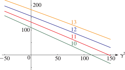
Antia (1993) gives minimax rational approximations for $\Gamma\left(s+1\right)F_{s}(x)$ , where $F_{s}(x)$ is the Fermi–Dirac integral (25.12.14), for the intervals $-\infty<x\leq 2$ and $2\leq x<\infty$ , with $s=-\frac{1}{2},\frac{1}{2},\frac{3}{2},\frac{5}{2}$ . For each $s$ there are three sets of approximations, with relative maximum errors $10^{-4},10^{-8},10^{-12}$ .

… ►

R. Barakat (1961) Evaluation of the incomplete gamma function of imaginary argument by Chebyshev polynomials. Math. Comp. 15 (73), pp. 7–11.

ⓘ

External Links:: FullText, MathReview (J. C. P. Miller), ZentralBlatt
Referenced by:: §8.7.
Encodings:: BibTeX

… ►

B. C. Berndt, S. Bhargava, and F. G. Garvan (1995) Ramanujan’s theories of elliptic functions to alternative bases. Trans. Amer. Math. Soc. 347 (11), pp. 4163–4244.

ⓘ

External Links:: ISSN 0002-9947, FullText, MathReview (J. Borwein), ZentralBlatt
Referenced by:: §15.8(v), §20.11(iii).
Encodings:: BibTeX

… ►

F. Bethuel (1998) Vortices in Ginzburg-Landau Equations. In Proceedings of the International Congress of Mathematicians, Vol. III (Berlin, 1998), pp. 11–19.

ⓘ

External Links:: ISSN 1431-0643, FullText, MathReview Entry, ZentralBlatt
Referenced by:: §17.17.
Encodings:: BibTeX

… ►

R. L. Bishop (1981) Rainbow over Woolsthorpe Manor. Notes and Records Roy. Soc. London 36 (1), pp. 3–11 (1 plate).

ⓘ

External Links:: ISSN 0035-9149, Document, MathReview
Referenced by:: Sidebar 9.SB1.
Encodings:: BibTeX

… ►

R. W. Butler and A. T. A. Wood (2002) Laplace approximations for hypergeometric functions with matrix argument. Ann. Statist. 30 (4), pp. 1155–1177.

ⓘ

External Links:: ISSN 0090-5364, Document, MathReview, ZentralBlatt
Referenced by:: §35.6(iv), §35.7(iv), §35.7(iv), §35.9.
Encodings:: BibTeX

…

… ►For information on tables published before 1961 see Fletcher et al. (1962, v. 1, §4) and Lebedev and Fedorova (1960, Chapters 11 and 14).

.2014年世界杯朝鲜战绩『网址:mxsty.cc』.世界杯1998假球-m6q3s2-2022年11月30日9时27分4秒

11—20 of 539 matching pages

11: 34.7 Basic Properties: $\mathit{9j}$ Symbol

12: Bibliography Y

13: 27.2 Functions

14: 28.6 Expansions for Small $q$

15: Bibliography G

16: 30.7 Graphics

17: 30 Spheroidal Wave Functions

Chapter 30 Spheroidal Wave Functions

18: 25.20 Approximations

19: Bibliography B

20: 24.20 Tables

$n$	$\phi\left(n\right)$	$d\left(n\right)$	$\sigma\left(n\right)$	$n$	$\phi\left(n\right)$	$d\left(n\right)$	$\sigma\left(n\right)$	$n$	$\phi\left(n\right)$	$d\left(n\right)$	$\sigma\left(n\right)$	$n$	$\phi\left(n\right)$	$d\left(n\right)$	$\sigma\left(n\right)$
…
3	2	2	4	16	8	5	31	29	28	2	30	42	12	8	96
4	2	3	7	17	16	2	18	30	8	8	72	43	42	2	44
5	4	2	6	18	6	6	39	31	30	2	32	44	20	6	84
…
11	10	2	12	24	8	8	60	37	36	2	38	50	20	6	93
…

$n$	$\phi\left(n\right)$	$d\left(n\right)$	$\sigma\left(n\right)$	$n$	$\phi\left(n\right)$	$d\left(n\right)$	$\sigma\left(n\right)$	$n$	$\phi\left(n\right)$	$d\left(n\right)$	$\sigma\left(n\right)$	$n$	$\phi\left(n\right)$	$d\left(n\right)$	$\sigma\left(n\right)$
…
3	2	2	4	16	8	5	31	29	28	2	30	42	12	8	96
4	2	3	7	17	16	2	18	30	8	8	72	43	42	2	44
5	4	2	6	18	6	6	39	31	30	2	32	44	20	6	84
…
11	10	2	12	24	8	8	60	37	36	2	38	50	20	6	93
…

.2014年世界杯朝鲜战绩『网址:mxsty.cc』.世界杯1998假球-m6q3s2-2022年11月30日9时27分4秒

11—20 of 539 matching pages

11: 34.7 Basic Properties: 9 ⁢ j Symbol

12: Bibliography Y

13: 27.2 Functions

14: 28.6 Expansions for Small q

15: Bibliography G

16: 30.7 Graphics

17: 30 Spheroidal Wave Functions

Chapter 30 Spheroidal Wave Functions

18: 25.20 Approximations

19: Bibliography B

20: 24.20 Tables

11: 34.7 Basic Properties: $\mathit{9j}$ Symbol

14: 28.6 Expansions for Small $q$

$n$	$\phi\left(n\right)$	$d\left(n\right)$	$\sigma\left(n\right)$	$n$	$\phi\left(n\right)$	$d\left(n\right)$	$\sigma\left(n\right)$	$n$	$\phi\left(n\right)$	$d\left(n\right)$	$\sigma\left(n\right)$	$n$	$\phi\left(n\right)$	$d\left(n\right)$	$\sigma\left(n\right)$
…
3	2	2	4	16	8	5	31	29	28	2	30	42	12	8	96
4	2	3	7	17	16	2	18	30	8	8	72	43	42	2	44
5	4	2	6	18	6	6	39	31	30	2	32	44	20	6	84
…
11	10	2	12	24	8	8	60	37	36	2	38	50	20	6	93
…