.历届世界杯金球奖数量『网址:mxsty.cc』.2017足球世界杯比赛-m6q3s2-2022年11月29日6时17分50秒.nzpvd1p5z
(0.003 seconds)
21—30 of 143 matching pages
21: 24.2 Definitions and Generating Functions
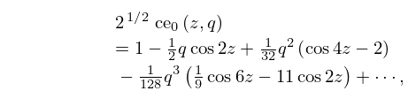
22: 28.6 Expansions for Small
23: 8.26 Tables
…
►
•
►
•
…
►
•
…
►
•
Pearson (1965) tabulates the function () for , to 7D, where rounds off to 1 to 7D; also for , to 5D.
Zhang and Jin (1996, Table 3.8) tabulates for , to 8D or 8S.
Pearson (1968) tabulates for , , with , to 7D.
Zhang and Jin (1996, Table 19.1) tabulates for , to 7D or 8S.
24: 6.19 Tables
…
►
•
…
►
•
Abramowitz and Stegun (1964, Chapter 5) includes , , , , ; , , , , ; , , , , ; , , , , ; , , . Accuracy varies but is within the range 8S–11S.
Zhang and Jin (1996, pp. 690–692) includes the real and imaginary parts of , , , 8S.
25: Bibliography G
…
►
Algorithm 292: Regular Coulomb wave functions.
Comm. ACM 9 (11), pp. 793–795.
►
Algorithm 363: Complex error function.
Comm. ACM 12 (11), pp. 635.
…
►
Some integrals involving three Bessel functions when their arguments satisfy the triangle inequalities.
J. Math. Phys. 25 (11), pp. 3350–3356.
…
►
Stirling number representation problems.
Proc. Amer. Math. Soc. 11 (3), pp. 447–451.
…
►
Theory of Painlevé’s equations.
Differ. Uravn. 11 (11), pp. 373–376 (Russian).
…
26: Bibliography S
…
►
On integral representations for Lamé and other special functions.
SIAM J. Math. Anal. 11 (4), pp. 702–723.
…
►
The Laplace transforms of products of Airy functions.
Dirāsāt Ser. B Pure Appl. Sci. 19 (2), pp. 7–11.
…
►
A simple approach to asymptotic expansions for Fourier integrals of singular functions.
Appl. Math. Comput. 216 (11), pp. 3378–3385.
…
►
Représentation asymptotique de la solution générale de l’équation de Mathieu-Hill.
Acad. Roy. Belg. Bull. Cl. Sci. (5) 51 (11), pp. 1415–1446.
…
►
Exact error terms in the asymptotic expansion of a class of integral transforms. I. Oscillatory kernels.
SIAM J. Math. Anal. 11 (5), pp. 828–841.
…
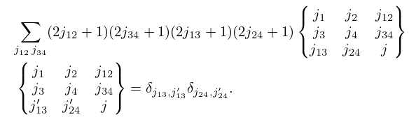
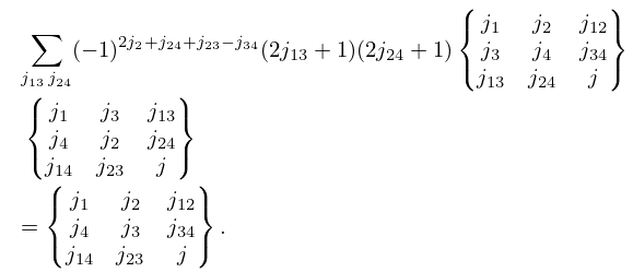
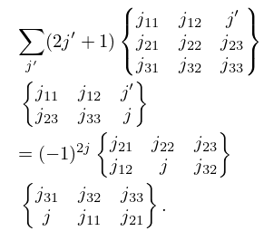
27: 34.7 Basic Properties: Symbol
28: 5.22 Tables
…
►Abramowitz and Stegun (1964, Chapter 6) tabulates , , , and for to 10D; and for to 10D; , , , , , , , and for to 8–11S; for to 20S.
Zhang and Jin (1996, pp. 67–69 and 72) tabulates , , , , , , , and for to 8D or 8S; for to 51S.
…
29: Bibliography Y
…
►
-squared discretizations of the continuum: Radial kinetic energy and the Coulomb Hamiltonian.
Phys. Rev. A 11 (4), pp. 1144–1156.
…
►
Software for interval arithmetic: A reasonably portable package.
ACM Trans. Math. Software 5 (1), pp. 50–63.
…
30: Bibliography C
…
►
Note on Nörlund’s polynomial
.
Proc. Amer. Math. Soc. 11 (3), pp. 452–455.
…
►
The fourth Painlevé equation and associated special polynomials.
J. Math. Phys. 44 (11), pp. 5350–5374.
…
►
Further formulas for calculating approximate values of the zeros of certain combinations of Bessel functions.
IEEE Trans. Microwave Theory Tech. 11 (6), pp. 546–547.
…
►
Validated computation of certain hypergeometric functions.
ACM Trans. Math. Software 38 (2), pp. Art. 11, 20.
…
►
Exact elliptic compactons in generalized Korteweg-de Vries equations.
Complexity 11 (6), pp. 30–34.
…
