���������������������������������V���ATV1819���e3y6
(0.000 seconds)
31—40 of 69 matching pages
31: 7.21 Physical Applications
…
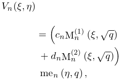
►Voigt functions , , can be regarded as the convolution of a Gaussian and a Lorentzian, and appear when the analysis of light (or particulate) absorption (or emission) involves thermal motion effects.
…
32: 12.11 Zeros
…
►If , then has no positive real zeros, and if , , then has a zero at .
…
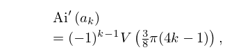
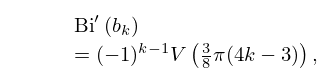
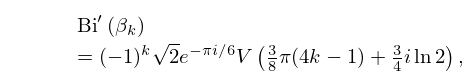
►For large negative values of the real zeros of , , , and can be approximated by reversion of the Airy-type asymptotic expansions of §§12.10(vii) and 12.10(viii).
…
33: 28.33 Physical Applications
…
►with , reduces to (28.32.2) with .
…The separated solutions must be -periodic in , and have the form
►
28.33.2
…
34: 18.39 Applications in the Physical Sciences
…
►The properties of determine whether the spectrum, this being the set of eigenvalues of , is discrete, continuous, or mixed, see §1.18.
…
►where is assumed to be independent of time.
…
►Now use spherical coordinates (1.5.16) with instead of , and assume the potential to be radial.
Then write instead of .
…
►Analogous to (18.39.8) the 3D time-independent Schrödinger equation with potential is
…
35: 10.17 Asymptotic Expansions for Large Argument
…
►
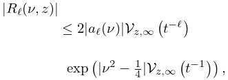
10.17.14
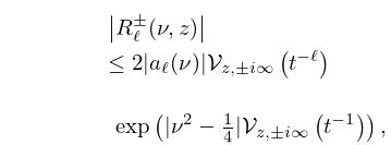
►where denotes the variational operator (2.3.6), and the paths of variation are subject to the condition that changes monotonically.
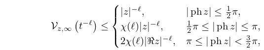
Bounds for are given by
►
10.17.15
…
►The bounds (10.17.15) also apply to in the conjugate sectors.
…
36: 18.9 Recurrence Relations and Derivatives
37: 10.40 Asymptotic Expansions for Large Argument
…
►
10.40.11
►where denotes the variational operator (§2.3(i)), and the paths of variation are subject to the condition that changes monotonically.
Bounds for are given by
►
10.40.12
…
38: 18.3 Definitions
…
►
…
39: 1.6 Vectors and Vector-Valued Functions
…
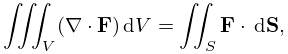
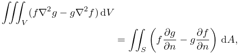
►Suppose is a piecewise smooth surface which forms the complete boundary of a bounded closed point set , and is oriented by its normal being outwards from .
…
►
1.6.58
…
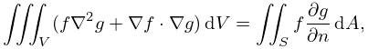
►
1.6.59
…
►
1.6.60
►where is the derivative of normal to the surface outwards from and is the unit outer normal vector.
…
