…
►
N
ν
2
(
x
)
ϕ
ν
′
(
x
)
=
2
(
x
2
−
ν
2
)
π
x
3
,
…
► As
x
→
∞
, with
ν
fixed and
μ
=
4
ν
2
,
…
►
10.18.20
−
(
2
k
−
3
)
!!
(
2
k
)
!!
(
μ
−
1
)
(
μ
−
9
)
⋯
(
μ
−
(
2
k
−
3
)
2
)
(
μ
−
(
2
k
+
1
)
(
2
k
−
1
)
2
)
(
2
x
)
2
k
,
k
≥
2
,
…
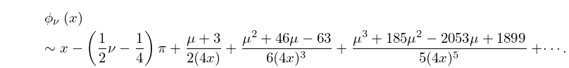
►
10.18.21
ϕ
ν
(
x
)
∼
x
−
(
1
2
ν
−
1
4
)
π
+
μ
+
3
2
(
4
x
)
+
μ
2
+
46
μ
−
63
6
(
4
x
)
3
+
μ
3
+
185
μ
2
−
2053
μ
+
1899
5
(
4
x
)
5
+
⋯
.
► In (
10.18.17 ) and (
10.18.18 ) the remainder after
n
terms does not exceed the
(
n
+
1
)
th term in absolute value and is of the same sign, provided that
n
>
ν
−
1
2
for (
10.18.17 ) and
−
3
2
≤
ν
≤
3
2
for (
10.18.18 ).
…
►
13.10.6
∫
0
∞
e
−
z
t
−
t
2
t
2
b
−
2
𝐌
(
a
,
b
,
t
2
)
d
t
=
1
2
π
−
1
2
Γ
(
b
−
1
2
)
U
(
b
−
1
2
,
a
+
1
2
,
1
4
z
2
)
,
ℜ
b
>
1
2
,
ℜ
z
>
0
,
…
►
13.10.9
1
2
π
i
∫
−
∞
(
0
+
)
e
t
z
t
−
a
U
(
a
,
b
,
y
/
t
)
d
t
=
2
z
1
2
(
2
a
−
b
−
1
)
y
1
2
(
1
−
b
)
Γ
(
a
)
Γ
(
a
−
b
+
1
)
K
b
−
1
(
2
z
y
)
,
ℜ
z
>
0
.
…
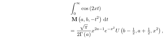
►
13.10.12
∫
0
∞
cos
(
2
x
t
)
𝐌
(
a
,
b
,
−
t
2
)
d
t
=
π
2
Γ
(
a
)
x
2
a
−
1
e
−
x
2
U
(
b
−
1
2
,
a
+
1
2
,
x
2
)
,
ℜ
a
>
0
.
…
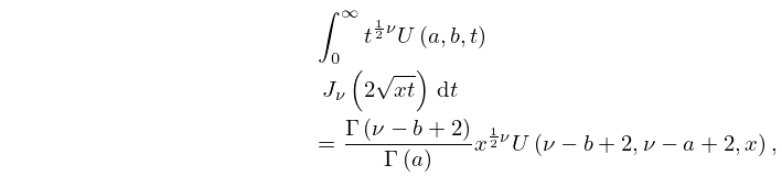
►
13.10.15
∫
0
∞
t
1
2
ν
U
(
a
,
b
,
t
)
J
ν
(
2
x
t
)
d
t
=
Γ
(
ν
−
b
+
2
)
Γ
(
a
)
x
1
2
ν
U
(
ν
−
b
+
2
,
ν
−
a
+
2
,
x
)
,
x
>
0
,
max
(
ℜ
b
−
2
,
−
1
)
<
ℜ
ν
<
2
ℜ
a
+
1
2
,
…
► For additional Hankel transforms and also other Bessel transforms see
Erdélyi et al. (1954b , §8.18) and
Oberhettinger (1972 , §§1.16 and 3.4.42–46 , 4.4.45–47, 5.94–97) .
…
…
► If any lower argument in a
6
j
symbol is
0
,
1
2
, or
1
, then the
6
j
symbol has a simple algebraic form.
…
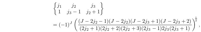
►
34.5.5
{
j
1
j
2
j
3
1
j
3
−
1
j
2
}
=
(
−
1
)
J
(
2
(
J
+
1
)
(
J
−
2
j
1
)
(
J
−
2
j
2
)
(
J
−
2
j
3
+
1
)
2
j
2
(
2
j
2
+
1
)
(
2
j
2
+
2
)
(
2
j
3
−
1
)
2
j
3
(
2
j
3
+
1
)
)
1
2
,
►
34.5.6
{
j
1
j
2
j
3
1
j
3
−
1
j
2
+
1
}
=
(
−
1
)
J
(
(
J
−
2
j
2
−
1
)
(
J
−
2
j
2
)
(
J
−
2
j
3
+
1
)
(
J
−
2
j
3
+
2
)
(
2
j
2
+
1
)
(
2
j
2
+
2
)
(
2
j
2
+
3
)
(
2
j
3
−
1
)
2
j
3
(
2
j
3
+
1
)
)
1
2
,
►
34.5.7
{
j
1
j
2
j
3
1
j
3
j
2
}
=
(
−
1
)
J
+
1
2
(
j
2
(
j
2
+
1
)
+
j
3
(
j
3
+
1
)
−
j
1
(
j
1
+
1
)
)
(
2
j
2
(
2
j
2
+
1
)
(
2
j
2
+
2
)
2
j
3
(
2
j
3
+
1
)
(
2
j
3
+
2
)
)
1
2
.
…
►
34.5.13
E
(
j
)
=
(
(
j
2
−
(
j
2
−
j
3
)
2
)
(
(
j
2
+
j
3
+
1
)
2
−
j
2
)
(
j
2
−
(
l
2
−
l
3
)
2
)
(
(
l
2
+
l
3
+
1
)
2
−
j
2
)
)
1
2
.
…
…
► The main functions treated in this chapter are the eigenvalues
a
ν
2
m
(
k
2
)
,
a
ν
2
m
+
1
(
k
2
)
,
b
ν
2
m
+
1
(
k
2
)
,
b
ν
2
m
+
2
(
k
2
)
, the Lamé functions
𝐸𝑐
ν
2
m
(
z
,
k
2
)
,
𝐸𝑐
ν
2
m
+
1
(
z
,
k
2
)
,
𝐸𝑠
ν
2
m
+
1
(
z
,
k
2
)
,
𝐸𝑠
ν
2
m
+
2
(
z
,
k
2
)
, and the Lamé polynomials
𝑢𝐸
2
n
m
(
z
,
k
2
)
,
𝑠𝐸
2
n
+
1
m
(
z
,
k
2
)
,
𝑐𝐸
2
n
+
1
m
(
z
,
k
2
)
,
𝑑𝐸
2
n
+
1
m
(
z
,
k
2
)
,
𝑠𝑐𝐸
2
n
+
2
m
(
z
,
k
2
)
,
𝑠𝑑𝐸
2
n
+
2
m
(
z
,
k
2
)
,
𝑐𝑑𝐸
2
n
+
2
m
(
z
,
k
2
)
,
𝑠𝑐𝑑𝐸
2
n
+
3
m
(
z
,
k
2
)
.
…
► Other notations that have been used are as follows:
Ince (1940a ) interchanges
a
ν
2
m
+
1
(
k
2
)
with
b
ν
2
m
+
1
(
k
2
)
.
The relation to the Lamé functions
L
c
ν
(
m
)
,
L
s
ν
(
m
)
of
Jansen (1977 ) is given by
…
►
𝐸𝑠
ν
2
m
+
2
(
z
,
k
2
)
=
s
ν
2
m
+
2
(
k
2
)
Es
ν
2
m
+
2
(
z
,
k
2
)
,
► where the positive factors
c
ν
m
(
k
2
)
and
s
ν
m
(
k
2
)
are determined by
…
…
►
§22.9(ii) Typical Identities of Rank 2
…
► These identities are
cyclic in the sense that each of the indices
m
,
n
in the first product of, for example, the form
s
m
,
p
(
4
)
s
n
,
p
(
4
)
are
simultaneously permuted in the cyclic order:
m
→
m
+
1
→
m
+
2
→
⋯
p
→
1
→
2
→
⋯
m
−
1
;
n
→
n
+
1
→
n
+
2
→
⋯
p
→
1
→
2
→
⋯
n
−
1
.
…
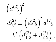
►
22.9.11
(
d
1
,
2
(
2
)
)
2
d
2
,
2
(
2
)
±
(
d
2
,
2
(
2
)
)
2
d
1
,
2
(
2
)
=
k
′
(
d
1
,
2
(
2
)
±
d
2
,
2
(
2
)
)
,
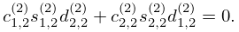
►
22.9.12
c
1
,
2
(
2
)
s
1
,
2
(
2
)
d
2
,
2
(
2
)
+
c
2
,
2
(
2
)
s
2
,
2
(
2
)
d
1
,
2
(
2
)
=
0
.
…
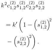
►
22.9.21
k
2
c
1
,
2
(
2
)
s
1
,
2
(
2
)
c
2
,
2
(
2
)
s
2
,
2
(
2
)
=
k
′
(
1
−
(
s
1
,
2
(
2
)
)
2
−
(
s
2
,
2
(
2
)
)
2
)
.
…
…
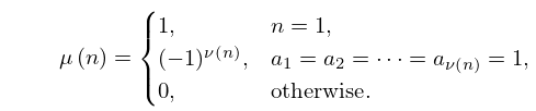
► where
p
1
,
p
2
,
…
,
p
ν
(
n
)
are the distinct prime factors of
n
, each exponent
a
r
is positive, and
ν
(
n
)
is the number of distinct primes dividing
n
.
…
► The
ϕ
(
n
)
numbers
a
,
a
2
,
…
,
a
ϕ
(
n
)
are relatively prime to
n
and distinct (mod
n
).
…It is the special case
k
=
2
of the function
d
k
(
n
)
that counts the number of ways of expressing
n
as the product of
k
factors, with the order of factors taken into account.
…
►
27.2.12
μ
(
n
)
=
{
1
,
n
=
1
,
(
−
1
)
ν
(
n
)
,
a
1
=
a
2
=
⋯
=
a
ν
(
n
)
=
1
,
0
,
otherwise
.
…
►
Table 27.2.2: Functions related to division.
►
►
