…
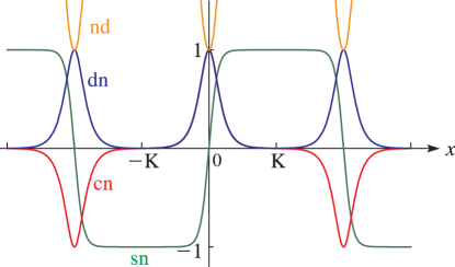
►►►Figure 22.3.4:
, , .
Magnify
…
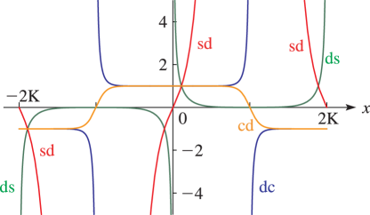
►►►Figure 22.3.8:
, , .
Magnify
…
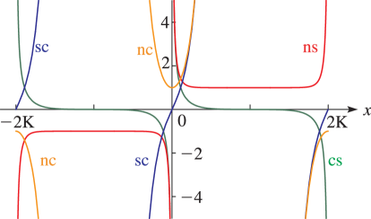
►►►Figure 22.3.12:
, , .
Magnify
…
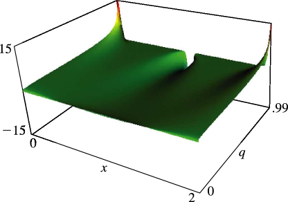
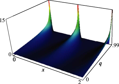
►In the graphics shown in this subsection height corresponds to the absolute value of the function and color to the phase.
…
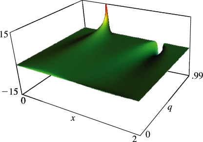
►In Figures 22.3.24 and 22.3.25, height corresponds to the absolute value of the function and color to the phase.
…
J. Faraut and A. Korányi (1994)Analysis on Symmetric Cones.
Oxford Mathematical Monographs, The Clarendon Press, Oxford University Press, Oxford-New York.
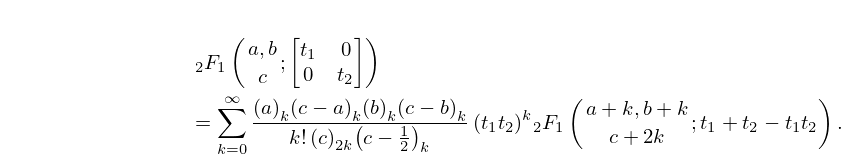
Originally the matrix in the argument of the Gaussian hypergeometric function
of matrix argument was written with round brackets. This
matrix has been rewritten with square brackets to be consistent with the rest
of the DLMF.
…
►Let (a) be orthogonally invariant, so that is a symmetric function of , the eigenvalues of the matrix argument ; (b) be analytic inin a neighborhood of ; (c) satisfy .
…
►Systems of partial differential equations for the (defined in §35.8) and functions of matrix argument can be obtained by applying (35.8.9) and (35.8.10) to (35.7.9).
…
►These approximations are in terms of elementary functions.
…
…
► 1924 in Croydon, U.
…degrees in mathematics from the University of London in 1945, 1948, and 1961, respectively.
…
►In 1992 he retired, and was appointed Professor Emeritus.
…
►In 1989 the conference “Asymptotic and Computational Analysis” was held in Winnipeg, Canada, in honor of Olver’s 65th birthday, with Proceedings published by Marcel Dekker in 1990.
…
►Most notably, he served as the Editor-in-Chief and Mathematics Editor of the onlineNIST Digital Library of Mathematical Functions and its 966-page print companion, the NIST Handbook of Mathematical Functions (Cambridge University Press, 2010).
…
…
►The results have been published in book form as the NIST Handbook of Mathematical Functions, by Cambridge University Press, and disseminated in the free electronic Digital Library of Mathematical Functions.
…Details of the early history of the DLMF Project are given in the Preface and on pp.
ix–xi in the NIST Handbook of Mathematical Functions.
…
►After the death in April 2013 of Frank W.
…
►They were selected as recognized leaders in the research communities interested in the mathematics and applications of special functions and orthogonal polynomials; in the presentation of mathematics reference information online and in handbooks; and in the presentation of mathematics on the web.
…
…
►A powerful way of computing the twelve Jacobian elliptic functions for real or complex values of both the argument and the modulus is to use the definitions in terms of theta functions given in §22.2, obtaining the theta functions via methods described in §20.14.
…
►By application of the transformations given in §§22.7(i) and 22.7(ii), or can always be made sufficently small to enable the approximations given in §22.10(ii) to be applied.
…
►From the first two terms in (22.10.6) we find .
Then by using (22.7.4) we have .
…
►Jacobi’s epsilon function can be computed from its representation (22.16.30) in terms of theta functions and complete elliptic integrals; compare §20.14.
…
►Figure 20.3.12:
, , .
Magnify3DHelp
…
►In the graphics shown in this subsection, height corresponds to the absolute value of the function and color to the phase.
…
►In the graphics shown in this subsection, height corresponds to the absolute value of the function and color to the phase.
…
…
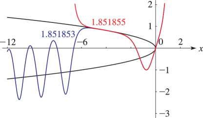
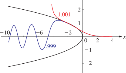
►►►Figure 32.3.3:
for and , .
…The parabola is shown in black.
Magnify►►►Figure 32.3.4:
for and , .
…The parabola is shown in black.
Magnify
…
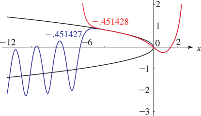
►►►Figure 32.3.6:
for with , .
…The parabola is shown in black.
Magnify
…
►If we set
in (32.3.2) and solve for , then
…
…
►They are denoted by , , , , respectively, arranged in ascending order of absolute value for
…
►They lie in the sectors and , and are denoted by , , respectively, in the former sector, and by , , in the conjugate sector, again arranged in ascending order of absolute value (modulus) for See §9.3(ii) for visualizations.
►For the distribution in
of the zeros of , where is an arbitrary complex constant, see Muraveĭ (1976) and Gil and Segura (2014).
…
►For error bounds for the asymptotic expansions of , , , and see Pittaluga and Sacripante (1991), and a conjecture given in Fabijonas and Olver (1999).
…
►Tables 9.9.3 and 9.9.4 give the corresponding results for the first ten complex zeros of and
in the upper half plane.
…
 ►
►
 ►
►
 ►
►
 ►
►
 ►
►
 ►
►
 ►
►
 ►
►
 ►
►
