%E8%8F%B2%E5%BE%8B%E5%AE%BE%E8%B5%8C%E5%9C%BA%E6%8E%92%E5%90%8D,%E8%8F%B2%E5%BE%8B%E5%AE%BE%E7%BD%91%E4%B8%8A%E8%B5%8C%E5%9C%BA,%E9%A9%AC%E5%B0%BC%E6%8B%89%E8%B5%8C%E5%9C%BA,%E3%80%90%E8%8F%B2%E5%BE%8B%E5%AE%BE%E8%B5%8C%E5%9C%BA%E7%BD%91%E5%9D%80%E2%88%B633kk66.com%E3%80%91%E8%8F%B2%E5%BE%8B%E5%AE%BE%E8%B5%8C%E5%9C%BA%E6%8B%9B%E8%81%98,%E8%8F%B2%E5%BE%8B%E5%AE%BE%E5%8D%9A%E5%BD%A9%E5%85%AC%E5%8F%B8,%E8%8F%B2%E5%BE%8B%E5%AE%BE%E5%8D%9A%E5%BD%A9%E7%BD%91%E7%AB%99,%E8%8F%B2%E5%BE%8B%E5%AE%BE%E8%B5%8C%E5%8D%9A%E7%BD%91%E7%AB%99,%E8%8F%B2%E5%BE%8B%E5%AE%BE%E8%B5%8C%E5%8D%9A%E5%B9%B3%E5%8F%B0,%E8%8F%B2%E5%BE%8B%E5%AE%BE%E8%B5%8C%E5%9C%BA%E5%9C%B0%E5%9D%80%E3%80%90%E5%A4%8D%E5%88%B6%E6%89%93%E5%BC%80%E2%88%B633kk66.com%E3%80%91

(0.056 seconds)

11—20 of 760 matching pages

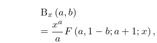
11: 8.17 Incomplete Beta Functions

… ►where, as in §5.12,

\mathrm{B}\left(a,b\right)

denotes the beta function: … ►For a historical profile of

\mathrm{B}_{x}\left(a,b\right)

see Dutka (1981). … ►

8.17.7

\mathrm{B}_{x}\left(a,b\right)=\frac{x^{a}}{a}F\left(a,1-b;a+1;x\right),

ⓘ

Symbols:: $F\left(\NVar{a},\NVar{b};\NVar{c};\NVar{z}\right)$ or $F\left({\NVar{a},\NVar{b}\atop\NVar{c}};\NVar{z}\right)$ : $={{}_{2}F_{1}}\left(\NVar{a},\NVar{b};\NVar{c};\NVar{z}\right)$ Gauss’ hypergeometric function, $\mathrm{B}_{\NVar{x}}\left(\NVar{a},\NVar{b}\right)$ : incomplete beta function, $a$ : parameter, $b$ : parameter and $x$ : variable
A&S Ref:: 6.6.8
Permalink:: http://dlmf.nist.gov/8.17.E7
Encodings:: pMML, png, TeX
See also:: Annotations for §8.17(ii), §8.17 and Ch.8

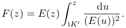
… ►For the hypergeometric function

F\left(a,b;c;z\right)

see §15.2(i). … ►Further integral representations can be obtained by combining the results given in §8.17(ii) with §15.6. …

12: 12.14 The Function $W\left(a,x\right)$

… ►For the modulus functions

\widetilde{F}(a,x)

and

\widetilde{G}(a,x)

see §12.14(x). … ►the branch of

\operatorname{ph}

being zero when

a=0

and defined by continuity elsewhere. … ►Other expansions, involving

\cos\left(\tfrac{1}{4}x^{2}\right)

and

\sin\left(\tfrac{1}{4}x^{2}\right)

, can be obtained from (12.4.3) to (12.4.6) by replacing

a

-ia

and

z

xe^{\ifrac{\pi i}{4}}

; see Miller (1955, p. 80), and also (12.14.15) and (12.14.16). … ►where

k

is defined in (12.14.5), and

\widetilde{F}(a,x)

(

>

0),

\widetilde{\theta}(a,x)

\widetilde{G}(a,x)

(

>

0), and

\widetilde{\psi}(a,x)

are real.

\widetilde{F}

\widetilde{G}

is the modulus and

\widetilde{\theta}

\widetilde{\psi}

is the corresponding phase. …

13: 19.24 Inequalities

… ►Other inequalities can be obtained by applying Carlson (1966, Theorems 2 and 3) to (19.16.20)–(19.16.23). … ►For

x>0

y>0

, and

x\neq y

, the complete cases of

R_{F}

and

R_{G}

satisfy … ►Inequalities for

R_{-a}\left(\mathbf{b};\mathbf{z}\right)

in Carlson (1966, Theorems 2 and 3) can be applied to (19.16.14)–(19.16.17). … ►Inequalities for

R_{C}\left(x,y\right)

and

R_{D}\left(x,y,z\right)

are included as special cases (see (19.16.6) and (19.16.5)). ►Other inequalities for

R_{F}\left(x,y,z\right)

are given in Carlson (1970). …

14: 19.5 Maclaurin and Related Expansions

… ►where

{{}_{2}F_{1}}

is the Gauss hypergeometric function (§§15.1 and 15.2(i)). …where

{F_{1}}\left(\alpha;\beta,\beta^{\prime};\gamma;x,y\right)

is an Appell function (§16.13). … ►Coefficients of terms up to

\lambda^{49}

are given in Lee (1990), along with tables of fractional errors in

K\left(k\right)

and

E\left(k\right)

0.1\leq k^{2}\leq 0.9999

, obtained by using 12 different truncations of (19.5.6) in (19.5.8) and (19.5.9). … ►Series expansions of

F\left(\phi,k\right)

and

E\left(\phi,k\right)

are surveyed and improved in Van de Vel (1969), and the case of

F\left(\phi,k\right)

is summarized in Gautschi (1975, §1.3.2). For series expansions of

\Pi\left(\phi,\alpha^{2},k\right)

when

|\alpha^{2}|<1

see Erdélyi et al. (1953b, §13.6(9)). …

15: 33.12 Asymptotic Expansions for Large $\eta$

… ►

33.12.3

{F_{0}'\left(\eta,\rho\right)\atop G_{0}'\left(\eta,\rho\right)}\sim-\pi^{1/2}% (2\eta)^{-1/6}\left\{{\operatorname{Ai}\left(x\right)\atop\operatorname{Bi}% \left(x\right)}\left(\frac{B_{1}^{\prime}+xA_{1}}{\mu}+\frac{B_{2}^{\prime}+xA% _{2}}{\mu^{2}}+\cdots\right)+{\operatorname{Ai}'\left(x\right)\atop% \operatorname{Bi}'\left(x\right)}\left(\frac{B_{1}+A_{1}^{\prime}}{\mu}+\frac{% B_{2}+A_{2}^{\prime}}{\mu^{2}}+\cdots\right)\right\},

ⓘ

Symbols:: $\operatorname{Ai}\left(\NVar{z}\right)$ : Airy function, $\operatorname{Bi}\left(\NVar{z}\right)$ : Airy function, $\sim$ : Poincaré asymptotic expansion, $\pi$ : the ratio of the circumference of a circle to its diameter, $G_{\NVar{\ell}}\left(\NVar{\eta},\NVar{\rho}\right)$ : irregular Coulomb radial function, $F_{\NVar{\ell}}\left(\NVar{\eta},\NVar{\rho}\right)$ : regular Coulomb radial function, $\rho$ : nonnegative real variable, $\eta$ : real parameter, $x$ : variable, $\mu$ : variable, $A_{j}$ : coefficients and $B_{j}$ : coefficients
A&S Ref:: 14.4.10
Permalink:: http://dlmf.nist.gov/33.12.E3
Encodings:: pMML, png, TeX
See also:: Annotations for §33.12(i), §33.12 and Ch.33

… ►

33.12.6

{F_{0}\left(\eta,2\eta\right)\atop{3^{-\ifrac{1}{2}}G_{0}\left(\eta,2\eta% \right)}}\sim\frac{\Gamma\left(\frac{1}{3}\right)\omega^{1/2}}{2\sqrt{\pi}}% \left(1\mp\frac{2}{35}\frac{\Gamma\left(\frac{2}{3}\right)}{\Gamma\left(\frac{% 1}{3}\right)}\frac{1}{\omega^{4}}-\frac{8}{2025}\frac{1}{\omega^{6}}\mp\frac{5% 792}{46\,06875}\frac{\Gamma\left(\frac{2}{3}\right)}{\Gamma\left(\frac{1}{3}% \right)}\frac{1}{\omega^{10}}-\cdots\right),

ⓘ

Symbols:: $\Gamma\left(\NVar{z}\right)$ : gamma function, $\sim$ : Poincaré asymptotic expansion, $\pi$ : the ratio of the circumference of a circle to its diameter, $G_{\NVar{\ell}}\left(\NVar{\eta},\NVar{\rho}\right)$ : irregular Coulomb radial function, $F_{\NVar{\ell}}\left(\NVar{\eta},\NVar{\rho}\right)$ : regular Coulomb radial function, $\eta$ : real parameter and $\omega$ : factor
Permalink:: http://dlmf.nist.gov/33.12.E6
Encodings:: pMML, png, TeX
See also:: Annotations for §33.12(i), §33.12 and Ch.33

►

33.12.7

{F_{0}'\left(\eta,2\eta\right)\atop{3^{-\ifrac{1}{2}}G_{0}'\left(\eta,2\eta% \right)}}\sim\frac{\Gamma\left(\frac{2}{3}\right)}{2\sqrt{\pi}\omega^{1/2}}% \left(\pm 1+\frac{1}{15}\frac{\Gamma\left(\frac{1}{3}\right)}{\Gamma\left(% \frac{2}{3}\right)}\frac{1}{\omega^{2}}\pm\frac{2}{14175}\frac{1}{\omega^{6}}+% \frac{1436}{23\,38875}\frac{\Gamma\left(\frac{1}{3}\right)}{\Gamma\left(\frac{% 2}{3}\right)}\frac{1}{\omega^{8}}\pm\cdots\right),

ⓘ

Symbols:: $\Gamma\left(\NVar{z}\right)$ : gamma function, $\sim$ : Poincaré asymptotic expansion, $\pi$ : the ratio of the circumference of a circle to its diameter, $G_{\NVar{\ell}}\left(\NVar{\eta},\NVar{\rho}\right)$ : irregular Coulomb radial function, $F_{\NVar{\ell}}\left(\NVar{\eta},\NVar{\rho}\right)$ : regular Coulomb radial function, $\eta$ : real parameter and $\omega$ : factor
Referenced by:: §33.12(i)
Permalink:: http://dlmf.nist.gov/33.12.E7
Encodings:: pMML, png, TeX
See also:: Annotations for §33.12(i), §33.12 and Ch.33

… ►For asymptotic expansions of

F_{\ell}\left(\eta,\rho\right)

and

G_{\ell}\left(\eta,\rho\right)

when

\eta\to\pm\infty

see Temme (2015, Chapter 31). … ►Then, by application of the results given in §§2.8(iii) and 2.8(iv), two sets of asymptotic expansions can be constructed for

F_{\ell}\left(\eta,\rho\right)

and

G_{\ell}\left(\eta,\rho\right)

when

\eta\to\infty

. …

16: 29.17 Other Solutions

… ►If (29.2.1) admits a Lamé polynomial solution

E

, then a second linearly independent solution

F

is given by ►

29.17.1

F(z)=E(z)\int_{\mathrm{i}{K^{\prime}}}^{z}\frac{\,\mathrm{d}u}{(E(u))^{2}}.

ⓘ

Symbols:: ${K^{\prime}}\left(\NVar{k}\right)$ : Legendre’s complementary complete elliptic integral of the first kind, $\,\mathrm{d}\NVar{x}$ : differential of $x$ , $\mathrm{i}$ : imaginary unit, $\int$ : integral, $z$ : complex variable and $k$ : real parameter
Permalink:: http://dlmf.nist.gov/29.17.E1
Encodings:: pMML, png, TeX
See also:: Annotations for §29.17(i), §29.17 and Ch.29

… ►They are algebraic functions of

\operatorname{sn}\left(z,k\right)

\operatorname{cn}\left(z,k\right)

, and

\operatorname{dn}\left(z,k\right)

, and have primitive period

8K

. …

17: 19.30 Lengths of Plane Curves

… ►

19.30.3

s/a=E\left(\phi,k\right)={R_{F}\left(c-1,c-k^{2},c\right)-\tfrac{1}{3}k^{2}R_{% D}\left(c-1,c-k^{2},c\right)},

ⓘ

Symbols:: $R_{D}\left(\NVar{x},\NVar{y},\NVar{z}\right)$ : elliptic integral symmetric in only two variables, $R_{F}\left(\NVar{x},\NVar{y},\NVar{z}\right)$ : symmetric elliptic integral of first kind, $E\left(\NVar{\phi},\NVar{k}\right)$ : Legendre’s incomplete elliptic integral of the second kind, $\phi$ : real or complex argument, $k$ : real or complex modulus and $s$ : arclength
Referenced by:: §19.30(i)
Permalink:: http://dlmf.nist.gov/19.30.E3
Encodings:: pMML, png, TeX
See also:: Annotations for §19.30(i), §19.30 and Ch.19

… ►Cancellation on the second right-hand side of (19.30.3) can be avoided by use of (19.25.10). … ►

19.30.5

L(a,b)=4aE\left(k\right)=8aR_{G}\left(0,b^{2}/a^{2},1\right)=8R_{G}\left(0,a^{% 2},b^{2}\right)=8abR_{G}\left(0,a^{-2},b^{-2}\right),

ⓘ

Symbols:: $R_{G}\left(\NVar{x},\NVar{y},\NVar{z}\right)$ : symmetric elliptic integral of second kind, $E\left(\NVar{k}\right)$ : Legendre’s complete elliptic integral of the second kind, $k$ : real or complex modulus and $L(a,b)$ : length
Referenced by:: §19.15, §19.24(i), §19.30(i), §19.33(i), §19.9(i)
Permalink:: http://dlmf.nist.gov/19.30.E5
Encodings:: pMML, png, TeX
See also:: Annotations for §19.30(i), §19.30 and Ch.19

… ►Let

a^{2}

and

b^{2}

be replaced respectively by

a^{2}+\lambda

and

b^{2}+\lambda

, where

\lambda\in(-b^{2},\infty)

, to produce a family of confocal ellipses. … ►For

s

in terms of

E\left(\phi,k\right)

F\left(\phi,k\right)

, and an algebraic term, see Byrd and Friedman (1971, p. 3). …

18: 16.25 Methods of Computation

… ►Instead a boundary-value problem needs to be formulated and solved. See §§3.6(vii), 3.7(iii), Olde Daalhuis and Olver (1998), Lozier (1980), and Wimp (1984, Chapters 7, 8).

19: 36 Integrals with Coalescing Saddles

…

20: 19.36 Methods of Computation

… ►If (19.36.1) is used instead of its first five terms, then the factor

(3r)^{-1/6}

in Carlson (1995, (2.2)) is changed to

(3r)^{-1/8}

. ►For both

R_{D}

and

R_{J}

the factor

(r/4)^{-1/6}

in Carlson (1995, (2.18)) is changed to

(r/5)^{-1/8}

when the following polynomial of degree 7 (the same for both) is used instead of its first seven terms: … ►Accurate values of

F\left(\phi,k\right)-E\left(\phi,k\right)

for

k^{2}

near 0 can be obtained from

R_{D}

by (19.2.6) and (19.25.13). … ►The incomplete integrals

R_{F}\left(x,y,z\right)

and

R_{G}\left(x,y,z\right)

can be computed by successive transformations in which two of the three variables converge quadratically to a common value and the integrals reduce to

R_{C}

, accompanied by two quadratically convergent series in the case of

R_{G}

; compare Carlson (1965, §§5,6). … ►

F\left(\phi,k\right)

can be evaluated by using (19.25.5). …

11—20 of 760 matching pages

11: 8.17 Incomplete Beta Functions

12: 12.14 The Function W ⁡ ( a , x )

13: 19.24 Inequalities

14: 19.5 Maclaurin and Related Expansions

15: 33.12 Asymptotic Expansions for Large η

16: 29.17 Other Solutions

17: 19.30 Lengths of Plane Curves

18: 16.25 Methods of Computation

19: 36 Integrals with Coalescing Saddles

20: 19.36 Methods of Computation

12: 12.14 The Function $W\left(a,x\right)$

15: 33.12 Asymptotic Expansions for Large $\eta$