%E7%BD%91%E4%B8%8A%E5%8D%9A%E5%BD%A9%E5%B9%B3%E5%8F%B0,%E7%BD%91%E4%B8%8A%E5%8D%9A%E5%BD%A9%E7%BD%91%E7%AB%99,%E3%80%90%E7%BD%91%E4%B8%8A%E5%8D%9A%E5%BD%A9%E5%9C%B0%E5%9D%80%E2%88%B622kk33.com%E3%80%91%E7%BD%91%E4%B8%8A%E5%8D%9A%E5%BD%A9%E8%AE%BA%E5%9D%9B,%E7%BD%91%E4%B8%8A%E5%8D%9A%E5%BD%A9%E5%85%AC%E5%8F%B8,%E7%BD%91%E4%B8%8A%E5%8D%9A%E5%BD%A9%E8%AE%BA%E5%9D%9B,%E7%BD%91%E4%B8%8A%E5%8D%9A%E5%BD%A9%E8%B5%84%E8%AE%AF,%E7%9C%9F%E4%BA%BA%E5%8D%9A%E5%BD%A9%E6%B8%B8%E6%88%8F,%E3%80%90%E5%8D%9A%E5%BD%A9%E7%BD%91%E5%9D%80%E2%88%B622kk33.com%E3%80%91%E7%BD%91%E5%9D%80Zg0ngCkEEkEAkfn

SearchAdvancedHelp

(0.063 seconds)

21—30 of 582 matching pages

21: 3.3 Interpolation

… ►where $C$ is a simple closed contour in $D$ described in the positive rotational sense and enclosing the points $z,z_1,z_2,\mathrm{\dots },z_n$. … ►and $A_k^n$ are the Lagrangian interpolation coefficients defined by … ►where ${\omega }_{n+1}(\zeta )$ is given by (3.3.3), and $C$ is a simple closed contour in $D$ described in the positive rotational sense and enclosing $z_0,z_1,\mathrm{\dots },z_n$. … ►By using this approximation to $x$ as a new point, $x_3=x$, and evaluating $\left[f_0,f_1,f_2,f_3\right]x=\mathrm{1.12388\hspace{0.33em}6190}$, we find that $x=-\mathrm{2.33810\hspace{0.33em}7409}$, with 9 correct digits. … ►Then by using $x_3$ in Newton’s interpolation formula, evaluating $\left[x_0,x_1,x_2,x_3\right]f=-\mathrm{0.26608\hspace{0.33em}28233}$ and recomputing $f^{\prime }(x)$, another application of Newton’s rule with starting value $x_3$ gives the approximation $x=\mathrm{2.33810\hspace{0.33em}7373}$, with 8 correct digits. …

22: 16.24 Physical Applications

… ►

§16.24(iii) $\mathit{3}j$, $\mathit{6}j$, and $\mathit{9}j$ Symbols

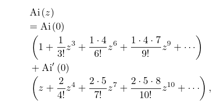
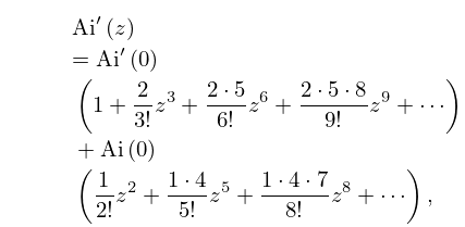
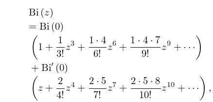
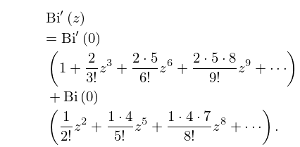
… ►They can be expressed as ${}_3{}^{}F_2^{}$ functions with unit argument. …These are balanced ${}_4{}^{}F_3^{}$ functions with unit argument. Lastly, special cases of the $\mathit{9}j$ symbols are ${}_5{}^{}F_4^{}$ functions with unit argument. …

23: 9.4 Maclaurin Series

… ►

9.4.1 $$\mathrm{Ai}\left(z\right)=\mathrm{Ai}\left(0\right)\left(1+\frac{1}{3!}{z}^3+\frac{1\cdot 4}{6!}{z}^6+\frac{1\cdot 4\cdot 7}{9!}{z}^9+\mathrm{\cdots }\right)+{\mathrm{Ai}}^{\prime }\left(0\right)\left(z+\frac{2}{4!}{z}^4+\frac{2\cdot 5}{7!}{z}^7+\frac{2\cdot 5\cdot 8}{10!}{z}^{10}+\mathrm{\cdots }\right),$$

ⓘ

Symbols:

$\mathrm{Ai}\left(z\right)$: Airy function, $!$: factorial (as in $n!$) and $z$: complex variable

Source:

Olver (1997b, p. 54)

A&S Ref:

10.4.2 (with 10.4.4 and 10.4.5)

Permalink:

http://dlmf.nist.gov/9.4.E1

Encodings:

pMML, png, TeX

See also:

Annotations for §9.4 and Ch.9

►

9.4.2 $${\mathrm{Ai}}^{\prime }\left(z\right)={\mathrm{Ai}}^{\prime }\left(0\right)\left(1+\frac{2}{3!}{z}^3+\frac{2\cdot 5}{6!}{z}^6+\frac{2\cdot 5\cdot 8}{9!}{z}^9+\mathrm{\cdots }\right)+\mathrm{Ai}\left(0\right)\left(\frac{1}{2!}{z}^2+\frac{1\cdot 4}{5!}{z}^5+\frac{1\cdot 4\cdot 7}{8!}{z}^8+\mathrm{\cdots }\right),$$

ⓘ

Symbols:

$\mathrm{Ai}\left(z\right)$: Airy function, $!$: factorial (as in $n!$) and $z$: complex variable

Proof sketch:

Use methods of Olver (1997b, p. 54).

Permalink:

http://dlmf.nist.gov/9.4.E2

Encodings:

pMML, png, TeX

See also:

Annotations for §9.4 and Ch.9

►

9.4.3 $$\mathrm{Bi}\left(z\right)=\mathrm{Bi}\left(0\right)\left(1+\frac{1}{3!}{z}^3+\frac{1\cdot 4}{6!}{z}^6+\frac{1\cdot 4\cdot 7}{9!}{z}^9+\mathrm{\cdots }\right)+{\mathrm{Bi}}^{\prime }\left(0\right)\left(z+\frac{2}{4!}{z}^4+\frac{2\cdot 5}{7!}{z}^7+\frac{2\cdot 5\cdot 8}{10!}{z}^{10}+\mathrm{\cdots }\right),$$

ⓘ

Symbols:

$\mathrm{Bi}\left(z\right)$: Airy function, $!$: factorial (as in $n!$) and $z$: complex variable

Proof sketch:

Use methods of Olver (1997b, p. 54).

A&S Ref:

10.4.3 (with 10.4.4 and 10.4.5)

Referenced by:

(9.12.15)

Permalink:

http://dlmf.nist.gov/9.4.E3

Encodings:

pMML, png, TeX

See also:

Annotations for §9.4 and Ch.9

►

9.4.4 $${\mathrm{Bi}}^{\prime }\left(z\right)={\mathrm{Bi}}^{\prime }\left(0\right)\left(1+\frac{2}{3!}{z}^3+\frac{2\cdot 5}{6!}{z}^6+\frac{2\cdot 5\cdot 8}{9!}{z}^9+\mathrm{\cdots }\right)+\mathrm{Bi}\left(0\right)\left(\frac{1}{2!}{z}^2+\frac{1\cdot 4}{5!}{z}^5+\frac{1\cdot 4\cdot 7}{8!}{z}^8+\mathrm{\cdots }\right).$$

ⓘ

Symbols:

$\mathrm{Bi}\left(z\right)$: Airy function, $!$: factorial (as in $n!$) and $z$: complex variable

Proof sketch:

Use methods of Olver (1997b, p. 54).

Permalink:

http://dlmf.nist.gov/9.4.E4

Encodings:

pMML, png, TeX

See also:

Annotations for §9.4 and Ch.9

24: Bibliography S

… ►

Orthogonal polynomials arising in the numerical evaluation of inverse Laplace transforms. Math. Tables Aids Comput. 9 (52), pp. 164–177.

ⓘ

External Links:

FullText, MathReview (S. C. van Veen), ZentralBlatt

Referenced by:

§3.5(viii).

Encodings:

BibTeX

… ►

Evaluation of associated Legendre functions off the cut and parabolic cylinder functions. Electron. Trans. Numer. Anal. 9, pp. 137–146.

ⓘ

Notes:

Orthogonal polynomials: numerical and symbolic algorithms (Leganés, 1998)

External Links:

ISSN 1068-9613, FullText, MathReview (Adam Marlewski), ZentralBlatt

Referenced by:

§14.30(i), 3rd item.

Encodings:

BibTeX

… ►

Parabolic Cylinder Functions and their Application in Symmetric Two-centre Shell Model. In Proceedings of the Conference on Mathematical Analysis and its Applications (Inst. Engrs., Mysore, 1977), Matscience Rep., Vol. 91, Aarhus, pp. P81–P89.

ⓘ

External Links:

MathReview

Referenced by:

§12.17.

Encodings:

BibTeX

… ►

A new Fortran program for the $9$-$j$ angular momentum coefficient. Comput. Phys. Comm. 56 (2), pp. 231–248.

ⓘ

External Links:

Document, ZentralBlatt

Referenced by:

§34.13.

Encodings:

BibTeX

… ►

An Introduction to Basic Fourier Series. Developments in Mathematics, Vol. 9, Kluwer Academic Publishers, Dordrecht.

ⓘ

External Links:

ISBN 1-4020-1221-7, MathReview (P. D. F. Ion), ZentralBlatt

Referenced by:

§17.3(i).

Encodings:

BibTeX

…

25: 19.36 Methods of Computation

… ►If (19.36.1) is used instead of its first five terms, then the factor ${(3r)}^{-1/6}$ in Carlson (1995, (2.2)) is changed to ${(3r)}^{-1/8}$. ►For both $R_D$ and $R_J$ the factor ${(r/4)}^{-1/6}$ in Carlson (1995, (2.18)) is changed to ${(r/5)}^{-1/8}$ when the following polynomial of degree 7 (the same for both) is used instead of its first seven terms: … ►All cases of $R_F$, $R_C$, $R_J$, and $R_D$ are computed by essentially the same procedure (after transforming Cauchy principal values by means of (19.20.14) and (19.2.20)). …Because of cancellations in (19.26.21) it is advisable to compute $R_G$ from $R_F$ and $R_D$ by (19.21.10) or else to use §19.36(ii). … ►Accurate values of $F(\varphi ,k)-E(\varphi ,k)$ for $k^2$ near 0 can be obtained from $R_D$ by (19.2.6) and (19.25.13). …

26: 16.26 Approximations

… ►For discussions of the approximation of generalized hypergeometric functions and the Meijer $G$-function in terms of polynomials, rational functions, and Chebyshev polynomials see Luke (1975, §§5.12 - 5.13) and Luke (1977b, Chapters 1 and 9).

27: 16.7 Relations to Other Functions

… ►For $\mathit{3}j$, $\mathit{6}j$, $\mathit{9}j$ symbols see Chapter 34. Further representations of special functions in terms of ${}_p{}^{}F_q^{}$ functions are given in Luke (1969a, §§6.2–6.3), and an extensive list of ${}_{q+1}{}^{}F_q^{}$ functions with rational numbers as parameters is given in Krupnikov and Kölbig (1997).

28: 34.13 Methods of Computation

… ►Methods of computation for $\mathit{3}j$ and $\mathit{6}j$ symbols include recursion relations, see Schulten and Gordon (1975a), Luscombe and Luban (1998), and Edmonds (1974, pp. 42–45, 48–51, 97–99); summation of single-sum expressions for these symbols, see Varshalovich et al. (1988, §§8.2.6, 9.2.1) and Fang and Shriner (1992); evaluation of the generalized hypergeometric functions of unit argument that represent these symbols, see Srinivasa Rao and Venkatesh (1978) and Srinivasa Rao (1981). ►For $\mathit{9}j$ symbols, methods include evaluation of the single-sum series (34.6.2), see Fang and Shriner (1992); evaluation of triple-sum series, see Varshalovich et al. (1988, §10.2.1) and Srinivasa Rao et al. (1989). …

29: 34.9 Graphical Method

§34.9 Graphical Method

… ►For specific examples of the graphical method of representing sums involving the $\mathit{3}j,\mathit{6}j$, and $\mathit{9}j$ symbols, see Varshalovich et al. (1988, Chapters 11, 12) and Lehman and O’Connell (1973, §3.3).

30: 34.10 Zeros

… ►Such zeros are called nontrivial zeros. ►For further information, including examples of nontrivial zeros and extensions to $\mathit{9}j$ symbols, see Srinivasa Rao and Rajeswari (1993, pp. 133–215, 294–295, 299–310).