%E5%85%AD%E5%90%88%E5%BD%A9%E8%A7%84%E5%88%99,%E5%85%AD%E5%90%88%E5%BD%A9%E6%8A%95%E6%B3%A8%E6%8A%80%E5%B7%A7,%E9%A6%99%E6%B8%AF%E5%85%AD%E5%90%88%E5%BD%A9%E9%A2%84%E6%B5%8B,%E3%80%90%E5%85%AD%E5%90%88%E5%BD%A9%E5%AE%98%E7%BD%91%E2%88%B622kk55.com%E3%80%91%E5%85%AD%E5%90%88%E5%BD%A9%E7%BD%91%E4%B8%8A%E6%8A%95%E6%B3%A8%E5%B9%B3%E5%8F%B0,%E6%BE%B3%E9%97%A8%E5%85%AD%E5%90%88%E5%BD%A9%E7%BD%91%E4%B8%8A%E6%8A%95%E6%B3%A8%E5%9C%B0%E5%9D%80,%E9%A6%99%E6%B8%AF%E5%85%AD%E5%90%88%E5%BD%A9%E9%A2%84%E6%B5%8B,%E3%80%90%E5%85%AD%E5%90%88%E5%BD%A9%E5%8D%9A%E5%BD%A9%E5%B9%B3%E5%8F%B0%E2%88%B622kk55.com%E3%80%91%E7%BD%91%E5%9D%80Zng0E0nAkC0gACg
(0.066 seconds)
21—30 of 758 matching pages
21: 14.33 Tables
…
►
•
►
•
►
•
…
Abramowitz and Stegun (1964, Chapter 8) tabulates for , , 5–8D; for , , 5–7D; and for , , 6–8D; and for , , 6S; and for , , 6S. (Here primes denote derivatives with respect to .)
Zhang and Jin (1996, Chapter 4) tabulates for , , 7D; for , , 8D; for , , 8S; for , , 8D; for , , , , 8S; for , , 8S; for , , , 5D; for , , 7S; for , , 8S. Corresponding values of the derivative of each function are also included, as are 6D values of the first 5 -zeros of and of its derivative for , .
Belousov (1962) tabulates (normalized) for , , , 6D.
22: Bibliography V
…
►
Integrating products of Bessel functions with an additional exponential or rational factor.
Comput. Phys. Comm. 178 (8), pp. 578–590.
…
►
Expansion of vacuum magnetic fields in toroidal harmonics.
Comput. Phys. Comm. 81 (1-2), pp. 74–90.
…
►
Certain summation formulae for -series.
J. Indian Math. Soc. (N.S.) 47 (1-4), pp. 71–85 (1986).
…
►
Dritter Beweis der die unvollständige Gammafunktion betreffenden Lochsschen Ungleichungen.
Österreich. Akad. Wiss. Math.-Natur. Kl. Sitzungsber. II 192 (1-3), pp. 83–91 (German).
…
►
Asymptotic expansion of the generalized hypergeometric function as for
.
Anal. Appl. (Singap.) 21 (2), pp. 535–545.
…
23: Bibliography S
…
►
Calculator function approximation.
Amer. Math. Monthly 90 (5), pp. 317–325.
…
►
A new Fortran 90 program to compute regular and irregular associated Legendre functions.
Comput. Phys. Comm. 181 (12), pp. 2091–2097.
…
►
The elliptical microstrip antenna with circular polarization.
IEEE Trans. Antennas and Propagation 29 (1), pp. 90–94.
…
►
Algorithm 814: Fortran 90 software for floating-point multiple precision arithmetic, gamma and related functions.
ACM Trans. Math. Software 27 (4), pp. 377–387.
…
►
Some results on the zeros of cylindrical functions and of their derivatives.
Rend. Sem. Mat. Univ. Politec. Torino 38 (1), pp. 67–85 (Italian. English summary).
…
24: Bibliography C
…
►
Generalized hypergeometric functions and the evaluation of scalar one-loop integrals in Feynman diagrams.
J. Comput. Appl. Math. 115 (1-2), pp. 93–99.
…
►
Reduction theorems for elliptic integrands with the square root of two quadratic factors.
J. Comput. Appl. Math. 118 (1-2), pp. 71–85.
…
►
Generalized incomplete gamma functions with applications.
J. Comput. Appl. Math. 55 (1), pp. 99–124.
…
►
Chebyshev polynomial expansions of complete elliptic integrals.
Math. Comp. 19 (90), pp. 249–259.
…
►
An algorithm for the machine calculation of complex Fourier series.
Math. Comp. 19 (90), pp. 297–301.
…
25: 29.20 Methods of Computation
…
►The normalization of Lamé functions given in §29.3(v) can be carried out by quadrature (§3.5).
…
►Initial approximations to the eigenvalues can be found, for example, from the asymptotic expansions supplied in §29.7(i).
…The Fourier series may be summed using Clenshaw’s algorithm; see §3.11(ii).
…
►These matrices are the same as those provided in §29.15(i) for the computation of Lamé polynomials with the difference that has to be chosen sufficiently large.
…
►Alternatively, the zeros can be found by locating the maximum of function in (29.12.11).
26: 26.12 Plane Partitions
…
►An equivalent definition is that a plane partition is a finite subset of with the property that if and , then must be an element of .
…It is useful to be able to visualize a plane partition as a pile of blocks, one block at each lattice point .
…
►We define the
box
as
…Then the number of plane partitions in is
…
►The number of symmetric plane partitions in is
…
27: 22.21 Tables
…
►Spenceley and Spenceley (1947) tabulates , , , , for and to 12D, or 12 decimals of a radian in the case of .
…
►Tables of theta functions (§20.15) can also be used to compute the twelve Jacobian elliptic functions by application of the quotient formulas given in §22.2.
28: Bibliography M
…
►
Two-point quasi-fractional approximations to the Airy function
.
J. Comput. Phys. 99 (2), pp. 337–340.
…
►
Foundations of Finite Precision Rational Arithmetic.
In Fundamentals of Numerical Computation (Computer-oriented
Numerical Analysis), G. Alefeld and R. D. Grigorieff (Eds.),
Comput. Suppl., Vol. 2, Vienna, pp. 85–111.
…
►
An improved calculation of the general elliptic integral of the second kind in the neighbourhood of
.
Numer. Math. 25 (1), pp. 99–101.
…
►
A class of generalized hypergeometric summations.
J. Comput. Appl. Math. 87 (1), pp. 79–85.
…
►
A new symmetry related to for classical basic hypergeometric series.
Adv. in Math. 57 (1), pp. 71–90.
…
29: 19.11 Addition Theorems
…
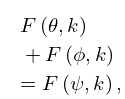
►
19.11.1
…
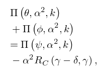
►
19.11.5
…
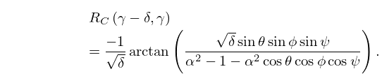
►
19.11.6_5
►Hence, care has to be taken with the multivalued functions in (19.11.5).
…
►
19.11.7
…
30: 25.16 Mathematical Applications
…
►In studying the distribution of primes , Chebyshev (1851) introduced a function (not to be confused with the digamma function used elsewhere in this chapter), given by
…
►where is given by (25.11.33).
►
is analytic for , and can be extended meromorphically into the half-plane for every positive integer by use of the relations
…
►For integer (), can be evaluated in terms of the zeta function:
…
►
has a simple pole with residue () at each odd negative integer , .
…
