%E4%BA%9A%E6%B4%B2%E5%8D%9A%E5%BD%A9%E5%B9%B3%E5%8F%B0,%E4%BA%9A%E6%B4%B2%E5%8D%9A%E5%BD%A9%E5%85%AC%E5%8F%B8,%E3%80%90%E4%BA%9A%E6%B4%B2%E5%8D%9A%E5%BD%A9%E7%BD%91%E5%9D%80%E2%88%B622kk33.com%E3%80%91%E4%BD%93%E8%82%B2%E5%8D%9A%E5%BD%A9%E5%85%AC%E5%8F%B8%E6%8E%92%E5%90%8D,%E6%9C%80%E5%A4%A7%E7%9A%84%E5%8D%9A%E5%BD%A9%E5%85%AC%E5%8F%B8,%E4%BA%9A%E6%B4%B2%E4%BD%93%E8%82%B2%E5%8D%9A%E5%BD%A9%E5%B9%B3%E5%8F%B0%E3%80%90%E7%BA%BF%E4%B8%8A%E5%8D%9A%E5%BD%A9%E2%88%B622kk33.com%E3%80%91%E7%BD%91%E5%9D%80ZEkEnBDkCBgfk0kC

(0.057 seconds)

11—20 of 601 matching pages

11: 34.10 Zeros

… ►Such zeros are called nontrivial zeros. ►For further information, including examples of nontrivial zeros and extensions to

\mathit{9j}

symbols, see Srinivasa Rao and Rajeswari (1993, pp. 133–215, 294–295, 299–310).

12: 34.13 Methods of Computation

… ►Methods of computation for

\mathit{3j}

and

\mathit{6j}

symbols include recursion relations, see Schulten and Gordon (1975a), Luscombe and Luban (1998), and Edmonds (1974, pp. 42–45, 48–51, 97–99); summation of single-sum expressions for these symbols, see Varshalovich et al. (1988, §§8.2.6, 9.2.1) and Fang and Shriner (1992); evaluation of the generalized hypergeometric functions of unit argument that represent these symbols, see Srinivasa Rao and Venkatesh (1978) and Srinivasa Rao (1981). ►For

\mathit{9j}

symbols, methods include evaluation of the single-sum series (34.6.2), see Fang and Shriner (1992); evaluation of triple-sum series, see Varshalovich et al. (1988, §10.2.1) and Srinivasa Rao et al. (1989). …

13: 34.7 Basic Properties: $\mathit{9j}$ Symbol

§34.7 Basic Properties: $\mathit{9j}$ Symbol

… ►

§34.7(ii) Symmetry

… ►

§34.7(iv) Orthogonality

… ►

§34.7(vi) Sums

… ►It constitutes an addition theorem for the

\mathit{9j}

symbol. …

14: 3.3 Interpolation

… ►where

C

is a simple closed contour in

D

described in the positive rotational sense and enclosing the points

z,z_{1},z_{2},\dots,z_{n}

. … ►and

A_{k}^{n}

are the Lagrangian interpolation coefficients defined by … ►where

\omega_{n+1}(\zeta)

is given by (3.3.3), and

C

is a simple closed contour in

{D}

described in the positive rotational sense and enclosing

z_{0},z_{1},\dots,z_{n}

. … ►By using this approximation to

x

as a new point,

x_{3}=x

, and evaluating

\left[f_{0},f_{1},f_{2},f_{3}\right]x=1.12388\;6190

, we find that

x=-2.33810\;7409

, with 9 correct digits. … ►Then by using

x_{3}

in Newton’s interpolation formula, evaluating

\left[x_{0},x_{1},x_{2},x_{3}\right]f=-0.26608\;28233

and recomputing

f^{\prime}(x)

, another application of Newton’s rule with starting value

x_{3}

gives the approximation

x=2.33810\;7373

, with 8 correct digits. …

15: 16.24 Physical Applications

… ►

§16.24(iii) $\mathit{3j}$ , $\mathit{6j}$ , and $\mathit{9j}$ Symbols

… ►They can be expressed as

{{}_{3}F_{2}}

functions with unit argument. …These are balanced

{{}_{4}F_{3}}

functions with unit argument. Lastly, special cases of the

\mathit{9j}

symbols are

{{}_{5}F_{4}}

functions with unit argument. …

16: 19.37 Tables

… ►Tabulated for

\phi=0(5^{\circ})90^{\circ}

k^{2}=0(.01)1

to 10D by Fettis and Caslin (1964). ►Tabulated for

\phi=0(1^{\circ})90^{\circ}

k^{2}=0(.01)1

to 7S by Beli͡akov et al. (1962). … ►Tabulated for

\phi=0(5^{\circ})90^{\circ}

k=0(.01)1

to 10D by Fettis and Caslin (1964). ►Tabulated for

\phi=0(5^{\circ})90^{\circ}

\operatorname{arcsin}k=0(1^{\circ})90^{\circ}

to 6D by Byrd and Friedman (1971), for

\phi=0(5^{\circ})90^{\circ}

\operatorname{arcsin}k=0(2^{\circ})90^{\circ}

and

5^{\circ}(10^{\circ})85^{\circ}

to 8D by Abramowitz and Stegun (1964, Chapter 17), and for

\phi=0(10^{\circ})90^{\circ}

\operatorname{arcsin}k=0(5^{\circ})90^{\circ}

to 9D by Zhang and Jin (1996, pp. 674–675). … ►Tabulated for

\phi=5^{\circ}(5^{\circ})80^{\circ}(2.5^{\circ})90^{\circ}

\alpha^{2}=-1(.1)-0.1,0.1(.1)1

k^{2}=0(.05)0.9(.02)1

to 10D by Fettis and Caslin (1964) (and warns of inaccuracies in Selfridge and Maxfield (1958) and Paxton and Rollin (1959)). …

17: 34.1 Special Notation

… ► ►►

$2j_{1},2j_{2},2j_{3},2l_{1},2l_{2},2l_{3}$	nonnegative integers.
…

►The main functions treated in this chapter are the Wigner

\mathit{3j},\mathit{6j},\mathit{9j}

symbols, respectively, … ►For other notations for

\mathit{3j}

\mathit{6j}

\mathit{9j}

symbols, see Edmonds (1974, pp. 52, 97, 104–105) and Varshalovich et al. (1988, §§8.11, 9.10, 10.10).

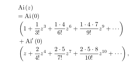
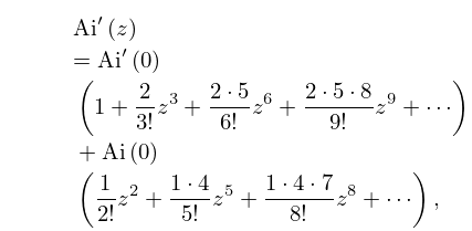
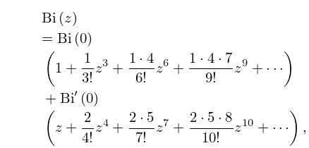
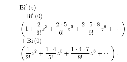
18: 9.4 Maclaurin Series

… ►

9.4.1

\operatorname{Ai}\left(z\right)=\operatorname{Ai}\left(0\right)\left(1+\frac{1% }{3!}z^{3}+\frac{1\cdot 4}{6!}z^{6}+\frac{1\cdot 4\cdot 7}{9!}z^{9}+\cdots% \right)+\operatorname{Ai}'\left(0\right)\left(z+\frac{2}{4!}z^{4}+\frac{2\cdot 5% }{7!}z^{7}+\frac{2\cdot 5\cdot 8}{10!}z^{10}+\cdots\right),

ⓘ

Symbols:: $\operatorname{Ai}\left(\NVar{z}\right)$ : Airy function, $!$ : factorial (as in $n!$ ) and $z$ : complex variable
Source:: Olver (1997b, p. 54)
A&S Ref:: 10.4.2 (with 10.4.4 and 10.4.5)
Permalink:: http://dlmf.nist.gov/9.4.E1
Encodings:: pMML, png, TeX
See also:: Annotations for §9.4 and Ch.9

►

9.4.2

\operatorname{Ai}'\left(z\right)=\operatorname{Ai}'\left(0\right)\left(1+\frac% {2}{3!}z^{3}+\frac{2\cdot 5}{6!}z^{6}+\frac{2\cdot 5\cdot 8}{9!}z^{9}+\cdots% \right)+\operatorname{Ai}\left(0\right)\left(\frac{1}{2!}z^{2}+\frac{1\cdot 4}% {5!}z^{5}+\frac{1\cdot 4\cdot 7}{8!}z^{8}+\cdots\right),

ⓘ

Symbols:: $\operatorname{Ai}\left(\NVar{z}\right)$ : Airy function, $!$ : factorial (as in $n!$ ) and $z$ : complex variable
Proof sketch:: Use methods of Olver (1997b, p. 54).
Permalink:: http://dlmf.nist.gov/9.4.E2
Encodings:: pMML, png, TeX
See also:: Annotations for §9.4 and Ch.9

►

9.4.3

\operatorname{Bi}\left(z\right)=\operatorname{Bi}\left(0\right)\left(1+\frac{1% }{3!}z^{3}+\frac{1\cdot 4}{6!}z^{6}+\frac{1\cdot 4\cdot 7}{9!}z^{9}+\cdots% \right)+\operatorname{Bi}'\left(0\right)\left(z+\frac{2}{4!}z^{4}+\frac{2\cdot 5% }{7!}z^{7}+\frac{2\cdot 5\cdot 8}{10!}z^{10}+\cdots\right),

ⓘ

Symbols:: $\operatorname{Bi}\left(\NVar{z}\right)$ : Airy function, $!$ : factorial (as in $n!$ ) and $z$ : complex variable
Proof sketch:: Use methods of Olver (1997b, p. 54).
A&S Ref:: 10.4.3 (with 10.4.4 and 10.4.5)
Referenced by:: (9.12.15)
Permalink:: http://dlmf.nist.gov/9.4.E3
Encodings:: pMML, png, TeX
See also:: Annotations for §9.4 and Ch.9

►

9.4.4

\operatorname{Bi}'\left(z\right)=\operatorname{Bi}'\left(0\right)\left(1+\frac% {2}{3!}z^{3}+\frac{2\cdot 5}{6!}z^{6}+\frac{2\cdot 5\cdot 8}{9!}z^{9}+\cdots% \right)+\operatorname{Bi}\left(0\right)\left(\frac{1}{2!}z^{2}+\frac{1\cdot 4}% {5!}z^{5}+\frac{1\cdot 4\cdot 7}{8!}z^{8}+\cdots\right).

ⓘ

Symbols:: $\operatorname{Bi}\left(\NVar{z}\right)$ : Airy function, $!$ : factorial (as in $n!$ ) and $z$ : complex variable
Proof sketch:: Use methods of Olver (1997b, p. 54).
Permalink:: http://dlmf.nist.gov/9.4.E4
Encodings:: pMML, png, TeX
See also:: Annotations for §9.4 and Ch.9

19: 3.2 Linear Algebra

… ►Assume that

\mathbf{A}

can be factored as in (3.2.5), but without partial pivoting. … ►where

\rho(\mathbf{A}\mathbf{A}^{\rm T})

is the largest of the absolute values of the eigenvalues of the matrix

\mathbf{A}\mathbf{A}^{\rm T}

; see §3.2(iv). … ►is called the characteristic polynomial of

\mathbf{A}

and its zeros are the eigenvalues of

\mathbf{A}

. … ►has the same eigenvalues as

\mathbf{A}

. … ►Many methods are available for computing eigenvalues; see Golub and Van Loan (1996, Chapters 7, 8), Trefethen and Bau (1997, Chapter 5), and Wilkinson (1988, Chapters 8, 9).

20: 26.10 Integer Partitions: Other Restrictions

… ►The set

\{n\geq 1\>|\>n\equiv\pm j\ \pmod{k}\}

is denoted by

A_{j,k}

. … ►Note that

p\left(\mathcal{D}^{\prime}3,n\right)\leq p\left(\mathcal{D}3,n\right)

, with strict inequality for

n\geq 9

. It is known that for

k>3

p\left(\mathcal{D}k,n\right)\geq p\left(\in\!A_{1,k+3},n\right)

, with strict inequality for

n

sufficiently large, provided that

k=2^{m}-1,m=3,4,5

, or

k\geq 32

; see Yee (2004). … ►where

I_{1}\left(x\right)

is the modified Bessel function (§10.25(ii)), and …The quantity

A_{k}(n)

is real-valued. …