Liouville%E2%80%93Green approximation theorem

SearchAdvancedHelp

(0.004 seconds)

41—50 of 289 matching pages

41: 10.31 Power Series

…

42: 3.4 Differentiation

… ►For formulas for derivatives with equally-spaced real nodes and based on Sinc approximations (§3.3(vi)), see Stenger (1993, §3.5). … ►The integral on the right-hand side can be approximated by the composite trapezoidal rule (3.5.2). … ►With the choice $r=k$ (which is crucial when $k$ is large because of numerical cancellation) the integrand equals ${\mathrm{e}}^k$ at the dominant points $\theta =0,2\pi$, and in combination with the factor $k^{-k}$ in front of the integral sign this gives a rough approximation to $1/k!$. … ►

Laplacian

… ►

Biharmonic Operator

…

43: 32.3 Graphics

… ►

►►

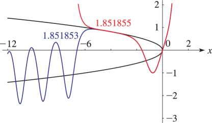
Figure 32.3.3: $w_k(x)$ for $-12\le x\le 0.73$ and $k=\mathrm{1.85185\hspace{0.33em}3}$, $\mathrm{1.85185\hspace{0.33em}5}$. The two graphs are indistinguishable when $x$ exceeds $-5.2$, approximately. … Magnify

… ►

►►

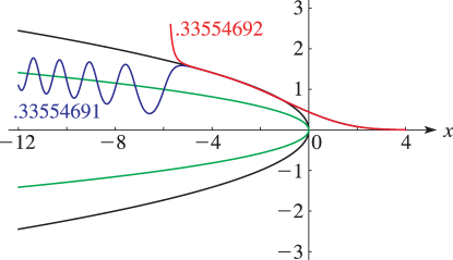
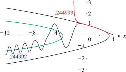
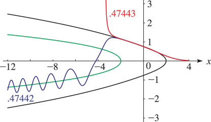
Figure 32.3.7: $u_k(x;-\frac{1}{2})$ for $-12\le x\le 4$ with $k=\mathrm{0.33554\hspace{0.33em}691}$, $\mathrm{0.33554\hspace{0.33em}692}$. …The parabolas $u^2+\frac{1}{2}x=0$, $u^2+\frac{1}{6}x=0$ are shown in black and green, respectively. Magnify

►

►►

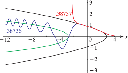
Figure 32.3.8: $u_k(x;\frac{1}{2})$ for $-12\le x\le 4$ with $k=0.47442$, $0.47443$. …The curves $u^2+\frac{1}{3}x\pm \frac{1}{6}\sqrt{x^2+12}=0$ are shown in green and black, respectively. Magnify

►

►►

Figure 32.3.9: $u_k(x;\frac{3}{2})$ for $-12\le x\le 4$ with $k=0.38736$, $0.38737$. …The curves $u^2+\frac{1}{3}x\pm \frac{1}{6}\sqrt{x^2+24}=0$ are shown in green and black, respectively. Magnify

►

►►

Figure 32.3.10: $u_k(x;\frac{5}{2})$ for $-12\le x\le 4$ with $k=\mathrm{0.24499\hspace{0.33em}2}$, $\mathrm{0.24499\hspace{0.33em}3}$. …The curves $u^2+\frac{1}{3}x\pm \frac{1}{6}\sqrt{x^2+36}=0$ are shown in green and black, respectively. Magnify

44: 2.3 Integrals of a Real Variable

… ►

§2.3(i) Integration by Parts

►Assume that the Laplace transform … ►For the Fourier integral … ►

§2.3(iv) Method of Stationary Phase

… ►

§2.3(v) Coalescing Peak and Endpoint: Bleistein’s Method

…

45: 32.8 Rational Solutions

… ►

32.8.3 $$w(z;3)=\frac{3z^2}{z^3+4}-\frac{6z^2(z^3+10)}{z^6+20z^3-80},$$

ⓘ

Symbols:

$z$: real

Permalink:

http://dlmf.nist.gov/32.8.E3

Encodings:

pMML, png, TeX

See also:

Annotations for §32.8(ii), §32.8 and Ch.32

►

32.8.4 $$w(z;4)=-\frac{1}{z}+\frac{6z^2(z^3+10)}{z^6+20z^3-80}-\frac{9z^5(z^3+40)}{z^9+60z^6+11200}.$$

ⓘ

Symbols:

$z$: real

Permalink:

http://dlmf.nist.gov/32.8.E4

Encodings:

pMML, png, TeX

See also:

Annotations for §32.8(ii), §32.8 and Ch.32

… ►

$$Q_3(z)=z^6+20z^3-80,$$

…

46: 10.34 Analytic Continuation

…

47: 12.12 Integrals

… ►For compendia of integrals see Erdélyi et al. (1953b, v. 2, pp. 121–122), Erdélyi et al. (1954a, b, v. 1, pp. 60–61, 115, 210–211, and 336; v. 2, pp. 76–80, 115, 151, 171, and 395–398), Gradshteyn and Ryzhik (2000, §7.7), Magnus et al. (1966, pp. 330–331), Marichev (1983, pp. 190–191), Oberhettinger (1974, pp. 144–145), Oberhettinger (1990, pp. 106–108 and 192), Oberhettinger and Badii (1973, pp. 181–185), Prudnikov et al. (1986b, pp. 36–37, 155–168, 243–246, 289–290, 327–328, 419–420, and 619), Prudnikov et al. (1992a, §3.11), and Prudnikov et al. (1992b, §3.11). …

48: 19.37 Tables

… ►Tabulated for $\varphi =5^{\circ }(5^{\circ }){80}^{\circ }({2.5}^{\circ }){90}^{\circ }$, ${\alpha }^2=-1(.1)-0.1,0.1(.1)1$, $k^2=0(.05)0.9(.02)1$ to 10D by Fettis and Caslin (1964) (and warns of inaccuracies in Selfridge and Maxfield (1958) and Paxton and Rollin (1959)). …

49: 1.6 Vectors and Vector-Valued Functions

… ►

Green’s Theorem

… ►

Stokes’s Theorem

… ►

Gauss’s (or Divergence) Theorem

… ►

Green’s Theorem (for Volume)

…

50: 26.6 Other Lattice Path Numbers

… ►

Table 26.6.1: Delannoy numbers $D(m,n)$.

► ►►►

$m$	$n$
	…
10	1	21	221	1561	8361	36365	1 34245	4 33905	12 56465	33 17445	80 97453

►

…