.2018年世界杯决赛裁判_『wn4.com_』1998年世界杯怎么了_w6n2c9o_2022年11月29日5时2分36秒_6ogsggucg_cc
(0.005 seconds)
41—50 of 789 matching pages
41: 3.7 Ordinary Differential Equations
…
►The path is partitioned at points labeled successively , with , .
…
►Write , , expand and in Taylor series (§1.10(i)) centered at , and apply (3.7.2).
…
►If, for example, , then on moving the contributions of and to the right-hand side of (3.7.13) the resulting system of equations is not tridiagonal, but can readily be made tridiagonal by annihilating the elements of that lie below the main diagonal and its two adjacent diagonals.
…
►The values are the eigenvalues and the corresponding solutions of the differential equation are the eigenfunctions.
…
►where and
…
42: 3.6 Linear Difference Equations
…
►Given numerical values of and , the solution of the equation
…These errors have the effect of perturbing the solution by unwanted small multiples of and of an independent solution , say.
…
►The unwanted multiples of now decay in comparison with , hence are of little consequence.
…
►The latter method is usually superior when the true value of is zero or pathologically small.
…
►beginning with .
…
43: 18.8 Differential Equations
44: 3.2 Linear Algebra
…
►where , , , and
…Forward elimination for solving then becomes ,
…and back substitution is , followed by
…
►Define the Lanczos vectors
and coefficients and by , a normalized vector (perhaps chosen randomly), , , and for by the recursive scheme
…
►Start with , vector such that , , .
…
45: 24.19 Methods of Computation
…
►Equations (24.5.3) and (24.5.4) enable and to be computed by recurrence.
…For example, the tangent numbers can be generated by simple recurrence relations obtained from (24.15.3), then (24.15.4) is applied.
…
►For other information see Chellali (1988) and Zhang and Jin (1996, pp. 1–11).
For algorithms for computing , , , and see Spanier and Oldham (1987, pp. 37, 41, 171, and 179–180).
►
§24.19(ii) Values of Modulo
…46: Bibliography O
…
►
Studies on the Painlevé equations. III. Second and fourth Painlevé equations, and
.
Math. Ann. 275 (2), pp. 221–255.
…
►
Hyperasymptotic solutions of higher order linear differential equations with a singularity of rank one.
Proc. Roy. Soc. London Ser. A 454, pp. 1–29.
…
►
Error bounds for stationary phase approximations.
SIAM J. Math. Anal. 5 (1), pp. 19–29.
…
►
Numerical solution of Riemann-Hilbert problems: Painlevé II.
Found. Comput. Math. 11 (2), pp. 153–179.
…
►
Algorithm 22: Riccati-Bessel functions of first and second kind.
Comm. ACM 3 (11), pp. 600–601.
…
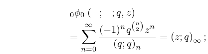
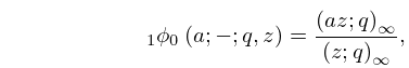
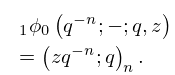
47: 17.5 Functions
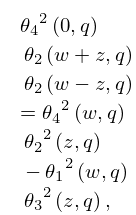
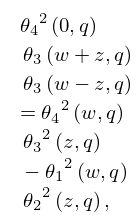
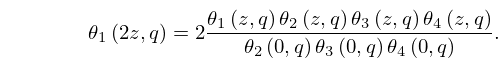
48: 20.7 Identities
49: 11.14 Tables
…
►
•
►
•
…
►
•
►
•
…
►
•
Abramowitz and Stegun (1964, Chapter 12) tabulates , , and for and , to 6D or 7D.
Agrest et al. (1982) tabulates and for and to 11D.
Abramowitz and Stegun (1964, Chapter 12) tabulates and for to 5D or 7D; , , and for to 6D.
Agrest et al. (1982) tabulates and for to 11D.
Agrest and Maksimov (1971, Chapter 11) defines incomplete Struve, Anger, and Weber functions and includes tables of an incomplete Struve function for , , and , together with surface plots.
50: 3.11 Approximation Techniques
…
►Beginning with , , we apply
…
►With , the last equations give as the solution of a system of linear equations.
…
►(3.11.29) is a system of linear equations for the coefficients .
…
►With this choice of and , the corresponding sum (3.11.32) vanishes.
…
►Two are endpoints: and ; the other points and are control points.
…
