.世界杯竞猜投注分析_『wn4.com_』中央1台世界杯时间表_w6n2c9o_2022年11月29日6时6分30秒_qsuoiwyqw_gov_hk

(0.007 seconds)

11—20 of 788 matching pages

11: 34.1 Special Notation

… ►

\begin{pmatrix}j_{1}&j_{2}&j_{3}\\ m_{1}&m_{2}&m_{3}\end{pmatrix},

►

\begin{Bmatrix}j_{1}&j_{2}&j_{3}\\ l_{1}&l_{2}&l_{3}\end{Bmatrix},

►

\begin{Bmatrix}j_{11}&j_{12}&j_{13}\\ j_{21}&j_{22}&j_{23}\\ j_{31}&j_{32}&j_{33}\end{Bmatrix}.

►An often used alternative to the

\mathit{3j}

symbol is the Clebsch–Gordan coefficient ►

34.1.1

\left(j_{1}\;m_{1}\;j_{2}\;m_{2}|j_{1}\;j_{2}\;j_{3}\,\,m_{3}\right)=(-1)^{j_{% 1}-j_{2}+m_{3}}(2j_{3}+1)^{\frac{1}{2}}\begin{pmatrix}j_{1}&j_{2}&j_{3}\\ m_{1}&m_{2}&-m_{3}\end{pmatrix};

ⓘ

Symbols:: $\begin{pmatrix}\NVar{j_{1}}&\NVar{j_{2}}&\NVar{j_{3}}\\ \NVar{m_{1}}&\NVar{m_{2}}&\NVar{m_{3}}\end{pmatrix}$ : $\mathit{3j}$ symbol and $j,j_{r}$ : non-negative integers or non-negative integers plus one half.
Sources:: Edmonds (1974, p. 46, Eq. (3.7.3)); Rotenberg et al. (1959, p. 1, Eq. (1.1a))
Permalink:: http://dlmf.nist.gov/34.1.E1
Encodings:: pMML, png, TeX
Clarification (effective with 1.0.15):: A wording change reflects that the Clebsch–Gordan coefficients are an alternative formulation of angular momentum problems, rather than alternative notation for the $\mathit{3j}$ . The sign of $m_{3}$ was changed for clarity.
See also:: Annotations for §34.1 and Ch.34

…

12: 24.2 Definitions and Generating Functions

… ►

B_{2n+1}=0

… ►

24.2.4

B_{n}=B_{n}\left(0\right),

ⓘ

Symbols:: $B_{\NVar{n}}$ : Bernoulli numbers, $B_{\NVar{n}}\left(\NVar{x}\right)$ : Bernoulli polynomials and $n$ : integer
A&S Ref:: 23.1.2
Referenced by:: (25.11.7)
Permalink:: http://dlmf.nist.gov/24.2.E4
Encodings:: pMML, png, TeX
See also:: Annotations for §24.2(i), §24.2 and Ch.24

… ►

Table 24.2.4: Euler numbers

E_{n}

► ►►

$n$	$E_{n}$
…

► ►

Table 24.2.5: Coefficients

b_{n,k}

of the Bernoulli polynomials

B_{n}\left(x\right)=\sum_{k=0}^{n}b_{n,k}x^{k}

► ►►

	$k$
…

► ►

Table 24.2.6: Coefficients

e_{n,k}

of the Euler polynomials

E_{n}\left(x\right)=\sum_{k=0}^{n}e_{n,k}x^{k}

► ►►

	$k$
…

►

13: 1.3 Determinants, Linear Operators, and Spectral Expansions

… ►The cofactor

A_{jk}

a_{jk}

is … ►For real-valued

a_{jk}

, … ►where

\omega_{1},\omega_{2},\dots,\omega_{n}

are the

n

th roots of unity (1.11.21). … ►If

D_{n}[a_{j,k}]

tends to a limit

L

n\to\infty

, then we say that the infinite determinant

D_{\infty}[a_{j,k}]

converges and

D_{\infty}[a_{j,k}]=L

. … ►The corresponding eigenvectors

\mathbf{a}_{1},\dots,\mathbf{a}_{n}

can be chosen such that they form a complete orthonormal basis in

\mathbf{E}_{n}

. …

14: 1.12 Continued Fractions

… ►

A_{n}

and

B_{n}

are called the

n

th (canonical) numerator and denominator respectively. … ►

b_{0}+\displaystyle{\cfrac{a_{1}}{b_{1}+\cfrac{a_{2}}{b_{2}+\cdots}}}

is equivalent to

b^{\prime}_{0}+\displaystyle{\cfrac{a^{\prime}_{1}}{b^{\prime}_{1}+\cfrac{a^{% \prime}_{2}}{b^{\prime}_{2}+\cdots}}}

if there is a sequence

\{d_{n}\}^{\infty}_{n=0}

d_{0}=1

d_{n}\neq 0

, such that … ►Define … ►The continued fraction

\displaystyle{\cfrac{a_{1}}{b_{1}+\cfrac{a_{2}}{b_{2}+\cdots}}}

converges when … ►Then the convergents

C_{n}

satisfy …

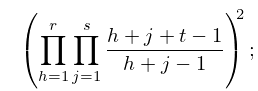
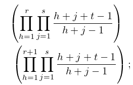
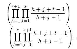
15: 26.12 Plane Partitions

… ►

26.12.9

\left(\prod_{h=1}^{r}\prod_{j=1}^{s}\frac{h+j+t-1}{h+j-1}\right)^{2};

ⓘ

Symbols:: $r$ : positive integer, $s$ : positive integer, $t$ : positive integer, $h$ : positive integer and $j$ : positive integer
Permalink:: http://dlmf.nist.gov/26.12.E9
Encodings:: pMML, png, TeX
See also:: Annotations for §26.12(i), §26.12 and Ch.26

… ►

26.12.10

\left(\prod_{h=1}^{r}\prod_{j=1}^{s}\frac{h+j+t-1}{h+j-1}\right)\*\left(\prod_% {h=1}^{r+1}\prod_{j=1}^{s}\frac{h+j+t-1}{h+j-1}\right);

ⓘ

Symbols:: $r$ : positive integer, $s$ : positive integer, $t$ : positive integer, $h$ : positive integer and $j$ : positive integer
Permalink:: http://dlmf.nist.gov/26.12.E10
Encodings:: pMML, png, TeX
See also:: Annotations for §26.12(i), §26.12 and Ch.26

… ►

26.12.11

\left(\prod_{h=1}^{r+1}\prod_{j=1}^{s}\frac{h+j+t-1}{h+j-1}\right)\*\left(% \prod_{h=1}^{r}\prod_{j=1}^{s+1}\frac{h+j+t-1}{h+j-1}\right).

ⓘ

Symbols:: $r$ : positive integer, $s$ : positive integer, $t$ : positive integer, $h$ : positive integer and $j$ : positive integer
Permalink:: http://dlmf.nist.gov/26.12.E11
Encodings:: pMML, png, TeX
See also:: Annotations for §26.12(i), §26.12 and Ch.26

… ►The notation

\sum_{\pi\subseteq B(r,s,t)}

denotes the sum over all plane partitions contained in

B(r,s,t)

, and

|\pi|

denotes the number of elements in

\pi

. … ►where

\sigma_{2}(j)

is the sum of the squares of the divisors of

j

. …

16: Bibliography

… ►

S. Ahmed and M. E. Muldoon (1980) On the zeros of confluent hypergeometric functions. III. Characterization by means of nonlinear equations. Lett. Nuovo Cimento (2) 29 (11), pp. 353–358.

ⓘ

External Links:: ISSN 0024-1318, MathReview (James M. Horner)
Referenced by:: §13.9(i).
Encodings:: BibTeX

… ►

D. E. Amos (1983c) Uniform asymptotic expansions for exponential integrals

E_{n}(x)

and Bickley functions

{\rm{K}i}_{n}(x)

. ACM Trans. Math. Software 9 (4), pp. 467–479.

ⓘ

External Links:: ISSN 0098-3500, Document, MathReview (Marietta J. Tretter), ZentralBlatt
Referenced by:: §10.43(iii).
Encodings:: BibTeX

… ►

K. Aomoto (1987) Special value of the hypergeometric function

{}_{3}F_{2}

and connection formulae among asymptotic expansions. J. Indian Math. Soc. (N.S.) 51, pp. 161–221.

ⓘ

External Links:: ISSN 0019-5839, MathReview (R. A. Askey), ZentralBlatt
Referenced by:: §16.4(iii).
Encodings:: BibTeX

… ►

V. I. Arnol’d (1972) Normal forms of functions near degenerate critical points, the Weyl groups

{A}_{k},{D}_{k},{E}_{k}

and Lagrangian singularities. Funkcional. Anal. i Priložen. 6 (4), pp. 3–25 (Russian).

ⓘ

Notes:: In Russian. English translation: Functional Anal. Appl., 6(1973), pp. 254–272.
External Links:: MathReview (G. R. Belickii), ZentralBlatt
Referenced by:: §36.2(i).
Encodings:: BibTeX

►

V. I. Arnol’d (1974) Normal forms of functions in the neighborhood of degenerate critical points. Uspehi Mat. Nauk 29 (2(176)), pp. 11–49 (Russian).

ⓘ

Notes:: Collection of articles dedicated to the memory of Ivan Georgievič Petrovskiĭ (1901–1973), I. In Russian. English translation: Russian Math. Surveys, 29(1974), no. 2, pp. 10–50.
External Links:: Document, MathReview (G. R. Belickii), ZentralBlatt
Referenced by:: §36.2(i).
Encodings:: BibTeX

…

17: 3.6 Linear Difference Equations

… ►Given numerical values of

w_{0}

and

w_{1}

, the solution

w_{n}

of the equation …These errors have the effect of perturbing the solution by unwanted small multiples of

w_{n}

and of an independent solution

g_{n}

, say. … ►The unwanted multiples of

g_{n}

now decay in comparison with

w_{n}

, hence are of little consequence. … ►The latter method is usually superior when the true value of

w_{0}

is zero or pathologically small. … ►beginning with

e_{0}=w_{0}

. …

18: 3.7 Ordinary Differential Equations

… ►The path is partitioned at

P+1

points labeled successively

z_{0},z_{1},\dots,z_{P}

, with

z_{0}=a

z_{P}=b

. … ►Write

\tau_{j}=z_{j+1}-z_{j}

j=0,1,\dots,P

, expand

w(z)

and

w^{\prime}(z)

in Taylor series (§1.10(i)) centered at

z=z_{j}

, and apply (3.7.2). … ►If, for example,

\beta_{0}=\beta_{1}=0

, then on moving the contributions of

w(z_{0})

and

w(z_{P})

to the right-hand side of (3.7.13) the resulting system of equations is not tridiagonal, but can readily be made tridiagonal by annihilating the elements of

\mathbf{A}_{P}

that lie below the main diagonal and its two adjacent diagonals. … ►The values

\lambda_{k}

are the eigenvalues and the corresponding solutions

w_{k}

of the differential equation are the eigenfunctions. … ►where

h=z_{n+1}-z_{n}

and …

19: 24.20 Tables

… ►Abramowitz and Stegun (1964, Chapter 23) includes exact values of

\sum_{k=1}^{m}k^{n}

m=1(1)100

n=1(1)10

;

\sum_{k=1}^{\infty}k^{-n}

\sum_{k=1}^{\infty}(-1)^{k-1}k^{-n}

\sum_{k=0}^{\infty}(2k+1)^{-n}

n=1,2,\dotsc

, 20D;

\sum_{k=0}^{\infty}(-1)^{k}(2k+1)^{-n}

n=1,2,\dotsc

, 18D. ►Wagstaff (1978) gives complete prime factorizations of

N_{n}

and

E_{n}

for

n=20(2)60

and

n=8(2)42

, respectively. … ►For information on tables published before 1961 see Fletcher et al. (1962, v. 1, §4) and Lebedev and Fedorova (1960, Chapters 11 and 14).

20: 3.2 Linear Algebra

… ►where

u_{j}=c_{j}

j=1,2,\dots,n-1

d_{1}=b_{1}

, and …Forward elimination for solving

\mathbf{A}\mathbf{x}=\mathbf{f}

then becomes

y_{1}=f_{1}

, …and back substitution is

x_{n}=y_{n}/d_{n}

, followed by … ►Define the Lanczos vectors

\mathbf{v}_{j}

and coefficients

\alpha_{j}

and

\beta_{j}

\mathbf{v}_{0}=\boldsymbol{{0}}

, a normalized vector

\mathbf{v}_{1}

(perhaps chosen randomly),

\alpha_{1}=\mathbf{v}_{1}^{\rm T}\mathbf{A}\mathbf{v}_{1}

\beta_{1}=0

, and for

j=1,2,\ldots,n-1

by the recursive scheme … ►Start with

\mathbf{v}_{0}=\boldsymbol{{0}}

, vector

\mathbf{v}_{1}

such that

\mathbf{v}_{1}^{\rm T}\mathbf{S}\mathbf{v}_{1}=1

\alpha_{1}=\mathbf{v}_{1}^{\rm T}\mathbf{A}\mathbf{v}_{1}

\beta_{1}=0

. …