29 Lamé Functions Lamé Polynomials 29.11 Lamé Wave Equation 29.13 Graphics

§29.12 Definitions

Keywords:: Lamé polynomials
Referenced by:: §29.12(i)
Permalink:: http://dlmf.nist.gov/29.12

§29.12(i) Elliptic-Function Form
§29.12(ii) Algebraic Form
§29.12(iii) Zeros

§29.12(i) Elliptic-Function Form

Notes:: See Arscott (1964b, Chapter 9).
Keywords:: Lamé functions, Lamé polynomials
Referenced by:: §29.14, §29.6(i)
Permalink:: http://dlmf.nist.gov/29.12.i

Throughout §§29.12–29.16 the order $\nu$ in the differential equation (29.2.1) is assumed to be a nonnegative integer.

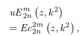
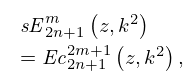
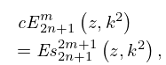
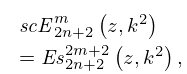
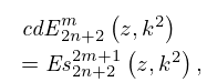
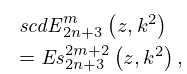
The Lamé functions $\mathop{\mathit{Ec}^{{m}}_{{\nu}}\/}\nolimits\!\left(z,k^{2}\right)$ , $m=0,1,\dots,\nu$ , and $\mathop{\mathit{Es}^{{m}}_{{\nu}}\/}\nolimits\!\left(z,k^{2}\right)$ , $m=1,2,\dots,\nu$ , are called the Lamé polynomials. There are eight types of Lamé polynomials, defined as follows:

29.12.1 $\mathop{\mathit{uE}^{{m}}_{{2n}}\/}\nolimits\!\left(z,k^{2}\right)=\mathop{% \mathit{Ec}^{{2m}}_{{2n}}\/}\nolimits\!\left(z,k^{2}\right),$

Defines:: $\mathop{\mathit{uE}^{{m}}_{{2n}}\/}\nolimits\!\left(z,k^{2}\right)$ : Lamé polynomial
Symbols:: $\mathop{\mathit{Ec}^{{m}}_{{\nu}}\/}\nolimits\!\left(z,k^{2}\right)$ : Lamé function, : nonnegative integer, : nonnegative integer, : complex variable and : real parameter
Referenced by:: §29.12(i)
Permalink:: http://dlmf.nist.gov/29.12.E1
Encodings:: TeX, pMML, png

29.12.2 $\mathop{\mathit{sE}^{{m}}_{{2n+1}}\/}\nolimits\!\left(z,k^{2}\right)=\mathop{% \mathit{Ec}^{{2m+1}}_{{2n+1}}\/}\nolimits\!\left(z,k^{2}\right),$

Defines:: $\mathop{\mathit{sE}^{{m}}_{{2n+1}}\/}\nolimits\!\left(z,k^{2}\right)$ : Lamé polynomial
Symbols:: $\mathop{\mathit{Ec}^{{m}}_{{\nu}}\/}\nolimits\!\left(z,k^{2}\right)$ : Lamé function, : nonnegative integer, : nonnegative integer, : complex variable and : real parameter
Permalink:: http://dlmf.nist.gov/29.12.E2
Encodings:: TeX, pMML, png

29.12.3 $\mathop{\mathit{cE}^{{m}}_{{2n+1}}\/}\nolimits\!\left(z,k^{2}\right)=\mathop{% \mathit{Es}^{{2m+1}}_{{2n+1}}\/}\nolimits\!\left(z,k^{2}\right),$

Defines:: $\mathop{\mathit{cE}^{{m}}_{{2n+1}}\/}\nolimits\!\left(z,k^{2}\right)$ : Lamé polynomial
Symbols:: $\mathop{\mathit{Es}^{{m}}_{{\nu}}\/}\nolimits\!\left(z,k^{2}\right)$ : Lamé function, : nonnegative integer, : nonnegative integer, : complex variable and : real parameter
Permalink:: http://dlmf.nist.gov/29.12.E3
Encodings:: TeX, pMML, png

29.12.4 $\mathop{\mathit{dE}^{{m}}_{{2n+1}}\/}\nolimits\!\left(z,k^{2}\right)=\mathop{% \mathit{Ec}^{{2m}}_{{2n+1}}\/}\nolimits\!\left(z,k^{2}\right),$

Defines:: $\mathop{\mathit{dE}^{{m}}_{{2n+1}}\/}\nolimits\!\left(z,k^{2}\right)$ : Lamé polynomial
Symbols:: $\mathop{\mathit{Ec}^{{m}}_{{\nu}}\/}\nolimits\!\left(z,k^{2}\right)$ : Lamé function, : nonnegative integer, : nonnegative integer, : complex variable and : real parameter
Permalink:: http://dlmf.nist.gov/29.12.E4
Encodings:: TeX, pMML, png

29.12.5 $\mathop{\mathit{scE}^{{m}}_{{2n+2}}\/}\nolimits\!\left(z,k^{2}\right)=\mathop{% \mathit{Es}^{{2m+2}}_{{2n+2}}\/}\nolimits\!\left(z,k^{2}\right),$

Defines:: $\mathop{\mathit{scE}^{{m}}_{{2n+2}}\/}\nolimits\!\left(z,k^{2}\right)$ : Lamé polynomial
Symbols:: $\mathop{\mathit{Es}^{{m}}_{{\nu}}\/}\nolimits\!\left(z,k^{2}\right)$ : Lamé function, : nonnegative integer, : nonnegative integer, : complex variable and : real parameter
Permalink:: http://dlmf.nist.gov/29.12.E5
Encodings:: TeX, pMML, png

29.12.6 $\mathop{\mathit{sdE}^{{m}}_{{2n+2}}\/}\nolimits\!\left(z,k^{2}\right)=\mathop{% \mathit{Ec}^{{2m+1}}_{{2n+2}}\/}\nolimits\!\left(z,k^{2}\right),$

Defines:: $\mathop{\mathit{sdE}^{{m}}_{{2n+2}}\/}\nolimits\!\left(z,k^{2}\right)$ : Lamé polynomial
Symbols:: $\mathop{\mathit{Ec}^{{m}}_{{\nu}}\/}\nolimits\!\left(z,k^{2}\right)$ : Lamé function, : nonnegative integer, : nonnegative integer, : complex variable and : real parameter
Permalink:: http://dlmf.nist.gov/29.12.E6
Encodings:: TeX, pMML, png

29.12.7 $\mathop{\mathit{cdE}^{{m}}_{{2n+2}}\/}\nolimits\!\left(z,k^{2}\right)=\mathop{% \mathit{Es}^{{2m+1}}_{{2n+2}}\/}\nolimits\!\left(z,k^{2}\right),$

Defines:: $\mathop{\mathit{cdE}^{{m}}_{{2n+2}}\/}\nolimits\!\left(z,k^{2}\right)$ : Lamé polynomial
Symbols:: $\mathop{\mathit{Es}^{{m}}_{{\nu}}\/}\nolimits\!\left(z,k^{2}\right)$ : Lamé function, : nonnegative integer, : nonnegative integer, : complex variable and : real parameter
Permalink:: http://dlmf.nist.gov/29.12.E7
Encodings:: TeX, pMML, png

29.12.8 $\mathop{\mathit{scdE}^{{m}}_{{2n+3}}\/}\nolimits\!\left(z,k^{2}\right)=\mathop% {\mathit{Es}^{{2m+2}}_{{2n+3}}\/}\nolimits\!\left(z,k^{2}\right),$

Defines:: $\mathop{\mathit{scdE}^{{m}}_{{2n+3}}\/}\nolimits\!\left(z,k^{2}\right)$ : Lamé polynomial
Symbols:: $\mathop{\mathit{Es}^{{m}}_{{\nu}}\/}\nolimits\!\left(z,k^{2}\right)$ : Lamé function, : nonnegative integer, : nonnegative integer, : complex variable and : real parameter
Referenced by:: §29.12(i)
Permalink:: http://dlmf.nist.gov/29.12.E8
Encodings:: TeX, pMML, png

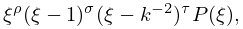
where $n=0,1,2,\dots$ , $m=0,1,2,\dots,n$ . These functions are polynomials in $\mathop{\mathrm{sn}\/}\nolimits\left(z,k\right)$ , $\mathop{\mathrm{cn}\/}\nolimits\left(z,k\right)$ , and $\mathop{\mathrm{dn}\/}\nolimits\left(z,k\right)$ . In consequence they are doubly-periodic meromorphic functions of .

The superscript on the left-hand sides of (29.12.1)–(29.12.8) agrees with the number of -zeros of each Lamé polynomial in the interval $(0,\!\mathop{K\/}\nolimits\!)$ , while is the number of -zeros in the open line segment from $\!\mathop{K\/}\nolimits\!$ to $\!\mathop{K\/}\nolimits\!+i\!\mathop{{K^{{\prime}}}\/}\nolimits\!$ .

The prefixes $\mathit{u}$ , $\mathit{s}$ , $\mathit{c}$ , $\mathit{d}$ , $\mathit{sc}$ , $\mathit{sd}$ , $\mathit{cd}$ , $\mathit{scd}$ indicate the type of the polynomial form of the Lamé polynomial; compare the 3rd and 4th columns in Table 29.12.1. In the fourth column the variable and modulus of the Jacobian elliptic functions have been suppressed, and $P({\mathop{\mathrm{sn}\/}\nolimits^{{2}}})$ denotes a polynomial of degree in ${\mathop{\mathrm{sn}\/}\nolimits^{{2}}}\left(z,k\right)$ (different for each type). For the determination of the coefficients of the ’s see §29.15(ii).

Table 29.12.1: Lamé polynomials.

$\nu$

eigenvalue

eigenfunction

polynomial

form

real

period

imag.

period

parity of

$w(z-\!\mathop{K\/}\nolimits\!)$

parity of

$w(z-\!\mathop{K\/}\nolimits\!-i\!\mathop{{K^{{\prime}}}\/}\nolimits\!)$

$\mathop{a^{{2m}}_{{\nu}}\/}\nolimits\!\left(k^{2}\right)$

$\mathop{\mathit{uE}^{{m}}_{{\nu}}\/}\nolimits\!\left(z,k^{2}\right)$

$P({\mathop{\mathrm{sn}\/}\nolimits^{{2}}})$

$2\!\mathop{K\/}\nolimits\!$

$2i\!\mathop{{K^{{\prime}}}\/}\nolimits\!$

even

$2n+1\;$

$\mathop{a^{{2m+1}}_{{\nu}}\/}\nolimits\!\left(k^{2}\right)$

$\mathop{\mathit{sE}^{{m}}_{{\nu}}\/}\nolimits\!\left(z,k^{2}\right)$

$\mathop{\mathrm{sn}\/}\nolimits P({\mathop{\mathrm{sn}\/}\nolimits^{{2}}})$

$4\!\mathop{K\/}\nolimits\!$

$2i\!\mathop{{K^{{\prime}}}\/}\nolimits\!$

odd

even

$2n+1\;$

$\mathop{b^{{2m+1}}_{{\nu}}\/}\nolimits\!\left(k^{2}\right)$

$\mathop{\mathit{cE}^{{m}}_{{\nu}}\/}\nolimits\!\left(z,k^{2}\right)$

$\mathop{\mathrm{cn}\/}\nolimits P({\mathop{\mathrm{sn}\/}\nolimits^{{2}}})$

$4\!\mathop{K\/}\nolimits\!$

$4i\!\mathop{{K^{{\prime}}}\/}\nolimits\!$

even

odd

even

$2n+1\;$

$\mathop{a^{{2m}}_{{\nu}}\/}\nolimits\!\left(k^{2}\right)$

$\mathop{\mathit{dE}^{{m}}_{{\nu}}\/}\nolimits\!\left(z,k^{2}\right)$

$\mathop{\mathrm{dn}\/}\nolimits P({\mathop{\mathrm{sn}\/}\nolimits^{{2}}})$

$2\!\mathop{K\/}\nolimits\!$

$4i\!\mathop{{K^{{\prime}}}\/}\nolimits\!$

even

odd

$2n+2\;$

$\mathop{b^{{2m+2}}_{{\nu}}\/}\nolimits\!\left(k^{2}\right)$

$\mathop{\mathit{scE}^{{m}}_{{\nu}}\/}\nolimits\!\left(z,k^{2}\right)$

$\mathop{\mathrm{sn}\/}\nolimits\mathop{\mathrm{cn}\/}\nolimits P({\mathop{% \mathrm{sn}\/}\nolimits^{{2}}})$

$2\!\mathop{K\/}\nolimits\!$

$4i\!\mathop{{K^{{\prime}}}\/}\nolimits\!$

odd

even

$2n+2\;$

$\mathop{a^{{2m+1}}_{{\nu}}\/}\nolimits\!\left(k^{2}\right)$

$\mathop{\mathit{sdE}^{{m}}_{{\nu}}\/}\nolimits\!\left(z,k^{2}\right)$

$\mathop{\mathrm{sn}\/}\nolimits\mathop{\mathrm{dn}\/}\nolimits P({\mathop{% \mathrm{sn}\/}\nolimits^{{2}}})$

$4\!\mathop{K\/}\nolimits\!$

$4i\!\mathop{{K^{{\prime}}}\/}\nolimits\!$

odd

even

odd

$2n+2\;$

$\mathop{b^{{2m+1}}_{{\nu}}\/}\nolimits\!\left(k^{2}\right)$

$\mathop{\mathit{cdE}^{{m}}_{{\nu}}\/}\nolimits\!\left(z,k^{2}\right)$

$\mathop{\mathrm{cn}\/}\nolimits\mathop{\mathrm{dn}\/}\nolimits P({\mathop{% \mathrm{sn}\/}\nolimits^{{2}}})$

$4\!\mathop{K\/}\nolimits\!$

$2i\!\mathop{{K^{{\prime}}}\/}\nolimits\!$

even

odd

$2n+3\;$

$\mathop{b^{{2m+2}}_{{\nu}}\/}\nolimits\!\left(k^{2}\right)$

$\mathop{\mathit{scdE}^{{m}}_{{\nu}}\/}\nolimits\!\left(z,k^{2}\right)$

$\mathop{\mathrm{sn}\/}\nolimits\mathop{\mathrm{cn}\/}\nolimits\mathop{\mathrm{% dn}\/}\nolimits P({\mathop{\mathrm{sn}\/}\nolimits^{{2}}})$

$2\!\mathop{K\/}\nolimits\!$

$2i\!\mathop{{K^{{\prime}}}\/}\nolimits\!$

odd

§29.12(ii) Algebraic Form

Notes:: See Arscott (1964b, §9.3.2).
Keywords:: Lamé polynomials
Permalink:: http://dlmf.nist.gov/29.12.ii

With the substitution $\xi={\mathop{\mathrm{sn}\/}\nolimits^{{2}}}\left(z,k\right)$ every Lamé polynomial in Table 29.12.1 can be written in the form

29.12.9 $\xi^{\rho}(\xi-1)^{\sigma}(\xi-k^{{-2}})^{\tau}P(\xi),$

Symbols:: : real parameter, $\xi={\mathop{\mathrm{sn}\/}\nolimits^{{2}}}\left(z,k\right)$ : substitution, (0 or $\tfrac{1}{2}$ ): parameter $\rho$ , (0 or $\tfrac{1}{2}$ ): parameter $\sigma$ , (0 or $\tfrac{1}{2}$ ): parameter $\tau$ and $P(\xi)$ : polynomial
Referenced by:: §29.12(ii), §29.12(iii)
Permalink:: http://dlmf.nist.gov/29.12.E9
Encodings:: TeX, pMML, png

where $\rho$ , $\sigma$ , $\tau$ are either 0 or $\frac{1}{2}$ . The polynomial $P(\xi)$ is of degree and has zeros (all simple) in and zeros (all simple) in $(1,k^{{-2}})$ . The functions (29.12.9) satisfy (29.2.2).

§29.12(iii) Zeros

Notes:: See Whittaker and Watson (1927, §23.46) and Arscott (1964b, §9.2.1).
Keywords:: Lamé polynomials
Referenced by:: §29.19(ii)
Permalink:: http://dlmf.nist.gov/29.12.iii

Let $\xi_{1},\xi_{2},\dots,\xi_{n}$ denote the zeros of the polynomial in (29.12.9) arranged according to

29.12.10 $0<\xi_{1}<\dots<\xi_{m}<1<\xi_{{m+1}}<\dots<\xi_{n}<k^{{-2}}.$

Symbols:: : nonnegative integer, : nonnegative integer, : real parameter and $\xi_{n}$ : zeros
Permalink:: http://dlmf.nist.gov/29.12.E10
Encodings:: TeX, pMML, png

Then the function

29.12.11 $g(t_{1},t_{2},\dots,t_{n})=\left(\prod_{{p=1}}^{n}t_{p}^{{\rho+\frac{1}{4}}}|t% _{p}-1|^{{\sigma+\frac{1}{4}}}(k^{{-2}}-t_{p})^{{\tau+\frac{1}{4}}}\right)% \prod_{{q<r}}(t_{r}-t_{q}),$

Symbols:: : nonnegative integer, : nonnegative integer, : real parameter, (0 or $\tfrac{1}{2}$ ): parameter $\rho$ , (0 or $\tfrac{1}{2}$ ): parameter $\sigma$ , (0 or $\tfrac{1}{2}$ ): parameter $\tau$ and $g(t_{1},\ldots,t_{n})$ : function
Referenced by:: §29.20(iii)
Permalink:: http://dlmf.nist.gov/29.12.E11
Encodings:: TeX, pMML, png

defined for $(t_{1},t_{2},\dots,t_{n})$ with

29.12.12 $0\leq t_{1}\leq\cdots\leq t_{m}\leq 1\leq t_{{m+1}}\leq\cdots\leq t_{n}\leq k^% {{-2}},$

Symbols:: : nonnegative integer, : nonnegative integer and : real parameter
Referenced by:: §29.12(iii)
Permalink:: http://dlmf.nist.gov/29.12.E12
Encodings:: TeX, pMML, png

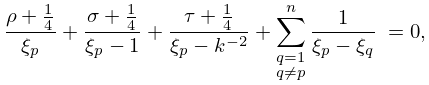
attains its absolute maximum iff $t_{j}=\xi_{j}$ , $j=1,2,\dots,n$ . Moreover,

29.12.13 ${\frac{\rho+\frac{1}{4}}{\xi_{p}}+\frac{\sigma+\frac{1}{4}}{\xi_{p}-1}+\frac{% \tau+\frac{1}{4}}{\xi_{p}-k^{{-2}}}+\sum_{{\substack{q=1\\ q\neq p}}}^{n}\frac{1}{\xi_{p}-\xi_{q}}=0},$ $p=1,2,\dots,n$ .

Symbols:: : nonnegative integer, : nonnegative integer, : real parameter, (0 or $\tfrac{1}{2}$ ): parameter $\rho$ , (0 or $\tfrac{1}{2}$ ): parameter $\sigma$ , (0 or $\tfrac{1}{2}$ ): parameter $\tau$ and $\xi_{n}$ : zeros
Referenced by:: §29.20(iii)
Permalink:: http://dlmf.nist.gov/29.12.E13
Encodings:: TeX, pMML, png

This result admits the following electrostatic interpretation: Given three point masses fixed at , , and $t=k^{{-2}}$ with positive charges $\rho+\tfrac{1}{4}$ , $\sigma+\tfrac{1}{4}$ , and $\tau+\tfrac{1}{4}$ , respectively, and movable point masses at $t_{1},t_{2},\dots,t_{n}$ arranged according to (29.12.12) with unit positive charges, the equilibrium position is attained when $t_{j}=\xi_{j}$ for $j=1,2,\dots,n$ .

© 2010–2013 NIST / Privacy Policy / Disclaimer / Feedback; Version 1.0.6; Release date 2013-05-06 Math-Image version (See MathML) . A Printed Companionis available. 29.11 Lamé Wave Equation 29.13 Graphics

§29.12 Definitions

Contents

§29.12(i) Elliptic-Function Form

§29.12(ii) Algebraic Form

§29.12(iii) Zeros