via non-classical orthogonal polynomials

(0.003 seconds)

11—20 of 338 matching pages

11: 35.12 Software

… ►Citations in the bulleted list refer to papers for which research software has been made available and can be downloaded via the Web. … ►

•

Demmel and Koev (2006). Computation of zonal polynomials in MATLAB.

… ►

•

Stembridge (1995). Maple software for zonal polynomials.

►For an algorithm to evaluate zonal polynomials, and an implementation of the algorithm in Maple by Zeilberger, see Lapointe and Vinet (1996).

12: Bibliography I

… ►

A. Iserles, P. E. Koch, S. P. Nørsett, and J. M. Sanz-Serna (1991) On polynomials orthogonal with respect to certain Sobolev inner products. J. Approx. Theory 65 (2), pp. 151–175.

ⓘ

External Links:: ISSN 0021-9045, Document, MathReview (R. A. Askey), ZentralBlatt
Referenced by:: §18.36(ii).
Encodings:: BibTeX

… ►

M. E. H. Ismail and D. R. Masson (1991) Two families of orthogonal polynomials related to Jacobi polynomials. Rocky Mountain J. Math. 21 (1), pp. 359–375.

ⓘ

External Links:: ISSN 0035-7596, MathReview (Joaquin Bustoz), ZentralBlatt
Referenced by:: §18.30(i).
Encodings:: BibTeX

… ►

M. E. H. Ismail (2000a) An electrostatics model for zeros of general orthogonal polynomials. Pacific J. Math. 193 (2), pp. 355–369.

ⓘ

External Links:: ISSN 0030-8730, FullText, MathReview (T. Erber), ZentralBlatt
Referenced by:: §18.39(v).
Encodings:: BibTeX

… ►

M. E. H. Ismail (2005) Classical and Quantum Orthogonal Polynomials in One Variable. Encyclopedia of Mathematics and its Applications, Vol. 98, Cambridge University Press, Cambridge.

ⓘ

External Links:: ISBN 978-0-521-78201-2; 0-521-78201-5, MathReview Entry, ZentralBlatt
Referenced by:: §1.4(v), Profile Mourad E.H. Ismail, Erratum (V1.0.20) for Chapter 18 Orthogonal Polynomials.
Encodings:: BibTeX

… ►

A. R. Its, A. S. Fokas, and A. A. Kapaev (1994) On the asymptotic analysis of the Painlevé equations via the isomonodromy method. Nonlinearity 7 (5), pp. 1291–1325.

ⓘ

External Links:: ISSN 0951-7715, Document, MathReview (Alexander Vladimirovich Kitaev), ZentralBlatt
Referenced by:: §32.11(iii).
Encodings:: BibTeX

…

13: 24.21 Software

… ►Citations in the bulleted list refer to papers for which research software has been made available and can be downloaded via the Web. … ►

§24.21(ii) $B_{n}$ , $B_{n}\left(x\right)$ , $E_{n}$ , and $E_{n}\left(x\right)$

…

14: 18.19 Hahn Class: Definitions

§18.19 Hahn Class: Definitions

… ►

Hahn, Krawtchouk, Meixner, and Charlier

►Tables 18.19.1 and 18.19.2 provide definitions via orthogonality and standardization (§§18.2(i), 18.2(iii)) for the Hahn polynomials

Q_{n}\left(x;\alpha,\beta,N\right)

, Krawtchouk polynomials

K_{n}\left(x;p,N\right)

, Meixner polynomials

M_{n}\left(x;\beta,c\right)

, and Charlier polynomials

C_{n}\left(x;a\right)

. … ►These polynomials are orthogonal on

(-\infty,\infty)

, and are defined as follows. …A special case of (18.19.8) is

w^{(1/2)}(x;\pi/2)=\frac{\pi}{\cosh\left(\pi x\right)}

15: 21.10 Methods of Computation

… ►

•

Belokolos et al. (1994, Chapter 5) and references therein. Here the Riemann surface is represented by the action of a Schottky group on a region of the complex plane. The same representation is used in Gianni et al. (1998).

►

•

Tretkoff and Tretkoff (1984). Here a Hurwitz system is chosen to represent the Riemann surface.

…

16: 18.30 Associated OP’s

… ►

§18.30(vi) Corecursive Orthogonal Polynomials

… ►

Numerator and Denominator Polynomials

… ►

§18.30(vii) Corecursive and Associated Monic Orthogonal Polynomials

►Defining associated orthogonal polynomials and their relationship to their corecursive counterparts is particularly simple via use of the recursion relations for the monic, rather than via those for the traditional polynomials. … ►

17: 18.40 Methods of Computation

… ►Orthogonal polynomials can be computed from their explicit polynomial form by Horner’s scheme (§1.11(i)). … ►

Stieltjes Inversion via (approximate) Analytic Continuation

… ►The bottom and top of the steps at the

x_{i}

are lower and upper bounds to

\int_{a}^{x_{i}}\,\mathrm{d}\mu(x)

as made explicit via the Chebyshev inequalities discussed by Shohat and Tamarkin (1970, pp. 42–43). … ►In what follows this is accomplished in two ways: i) via the Lagrange interpolation of §3.3(i) ; and ii) by constructing a pointwise continued fraction, or PWCF, as follows: …where the coefficients are defined recursively via

a_{1}=\frac{x_{1,N}}{x_{2,N}}-1

, and …

18: 22.18 Mathematical Applications

… ►

§22.18(i) Lengths and Parametrization of Plane Curves

… ►

§22.18(iii) Uniformization and Other Parametrizations

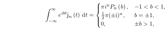
… ► … ►Algebraic curves of the form

y^{2}=P(x)

, where

P

is a nonsingular polynomial of degree 3 or 4 (see McKean and Moll (1999, §1.10)), are elliptic curves, which are also considered in §23.20(ii). …The existence of this group structure is connected to the Jacobian elliptic functions via the differential equation (22.13.1). …

19: 10.59 Integrals

… ►

10.59.1

\int_{-\infty}^{\infty}e^{ibt}\mathsf{j}_{n}\left(t\right)\,\mathrm{d}t=\begin% {cases}\pi i^{n}P_{n}\left(b\right),&-1<b<1,\\ \frac{1}{2}\pi(\pm\mathrm{i})^{n},&b=\pm 1,\\ 0,&\pm b>1,\end{cases}

ⓘ

Symbols:: $P_{\NVar{n}}\left(\NVar{x}\right)$ : Legendre polynomial, $\pi$ : the ratio of the circumference of a circle to its diameter, $\,\mathrm{d}\NVar{x}$ : differential of $x$ , $\mathrm{e}$ : base of natural logarithm, $\mathrm{i}$ : imaginary unit, $\int$ : integral, $\mathsf{j}_{\NVar{n}}\left(\NVar{z}\right)$ : spherical Bessel function of the first kind and $n$ : integer
A&S Ref:: 11.4.26
Referenced by:: §10.59
Permalink:: http://dlmf.nist.gov/10.59.E1
Encodings:: pMML, png, TeX
See also:: Annotations for §10.59 and Ch.10

►where

P_{n}

is the Legendre polynomial (§18.3). …

20: 31.8 Solutions via Quadratures

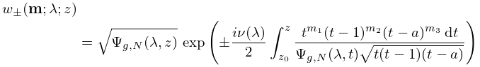
§31.8 Solutions via Quadratures

… ►

31.8.2

w_{\pm}(\mathbf{m};\lambda;z)=\sqrt{\Psi_{g,N}(\lambda,z)}\*\exp\left(\pm\frac% {i\nu(\lambda)}{2}\int_{z_{0}}^{z}\frac{t^{m_{1}}(t-1)^{m_{2}}(t-a)^{m_{3}}\,% \mathrm{d}t}{\Psi_{g,N}(\lambda,t)\sqrt{t(t-1)(t-a)}}\right)

ⓘ

Symbols:: $\,\mathrm{d}\NVar{x}$ : differential of $x$ , $\exp\NVar{z}$ : exponential function, $\mathrm{i}$ : imaginary unit, $\int$ : integral, $z$ : complex variable, $\nu$ : real or complex parameter, $m$ : nonnegative integer, $a$ : complex parameter, $\lambda=-4q$ , $\Psi_{g,N}(\lambda,z)$ : polynomial, $g$ : degree of $\lambda$ and $N$ : degree of $z$
Referenced by:: §31.8
Permalink:: http://dlmf.nist.gov/31.8.E2
Encodings:: pMML, png, TeX
See also:: Annotations for §31.8 and Ch.31

… ►Here

\Psi_{g,N}(\lambda,z)

is a polynomial of degree

g

\lambda

and of degree

N=m_{0}+m_{1}+m_{2}+m_{3}

z

, that is a solution of the third-order differential equation satisfied by a product of any two solutions of Heun’s equation. … ►When

\lambda=-4q

approaches the ends of the gaps, the solution (31.8.2) becomes the corresponding Heun polynomial. … ►The solutions in this section are finite-term Liouvillean solutions which can be constructed via Kovacic’s algorithm; see §31.14(ii).