values at z=0

SearchAdvancedHelp

(0.013 seconds)

31—40 of 144 matching pages

31: 9.19 Approximations

… ►

Martín et al. (1992) provides two simple formulas for approximating $\mathrm{Ai}\left(x\right)$ to graphical accuracy, one for , the other for .

►

Moshier (1989, §6.14) provides minimax rational approximations for calculating $\mathrm{Ai}\left(x\right)$, ${\mathrm{Ai}}^{\prime }\left(x\right)$, $\mathrm{Bi}\left(x\right)$, ${\mathrm{Bi}}^{\prime }\left(x\right)$. They are in terms of the variable $\zeta$, where $\zeta =\frac{2}{3}{x}^{3/2}$ when $x$ is positive, $\zeta =\frac{2}{3}{(-x)}^{3/2}$ when $x$ is negative, and $\zeta =0$ when $x=0$. The approximations apply when , that is, when or . The precision in the coefficients is 21S.

… ►These expansions are for real arguments $x$ and are supplied in sets of four for each function, corresponding to intervals , $a\le x\le 0$, $0\le x\le b$, . … ►

Corless et al. (1992) describe a method of approximation based on subdividing $ℂ$ into a triangular mesh, with values of $\mathrm{Ai}\left(z\right)$, ${\mathrm{Ai}}^{\prime }\left(z\right)$ stored at the nodes. $\mathrm{Ai}\left(z\right)$ and ${\mathrm{Ai}}^{\prime }\left(z\right)$ are then computed from Taylor-series expansions centered at one of the nearest nodes. The Taylor coefficients are generated by recursion, starting from the stored values of $\mathrm{Ai}\left(z\right)$, ${\mathrm{Ai}}^{\prime }\left(z\right)$ at the node. Similarly for $\mathrm{Bi}\left(z\right)$, ${\mathrm{Bi}}^{\prime }\left(z\right)$.

… ►

MacLeod (1994) supplies Chebyshev-series expansions to cover $\mathrm{Gi}\left(x\right)$ for and $\mathrm{Hi}\left(x\right)$ for . The Chebyshev coefficients are given to 20D.

32: 4.3 Graphics

… ►

►►

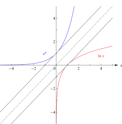
Figure 4.3.1: $\ln x$ and ${\mathrm{e}}^x$. Parallel tangent lines at $(1,0)$ and $(0,1)$ make evident the mirror symmetry across the line $y=x$, demonstrating the inverse relationship between the two functions. Magnify

… ►Figure 4.3.2 illustrates the conformal mapping of the strip onto the whole $w$-plane cut along the negative real axis, where $w={\mathrm{e}}^z$ and $z=\ln w$ (principal value). …Lines parallel to the real axis in the $z$-plane map onto rays in the $w$-plane, and lines parallel to the imaginary axis in the $z$-plane map onto circles centered at the origin in the $w$-plane. In the labeling of corresponding points $r$ is a real parameter that can lie anywhere in the interval $(0,\mathrm{\infty })$. 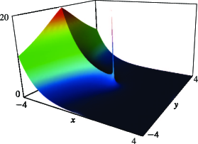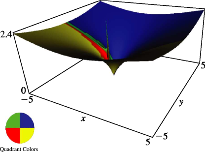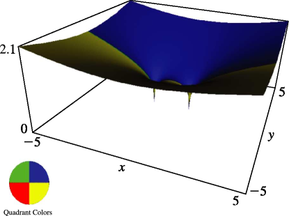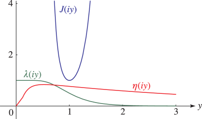… ►In the graphics shown in this subsection height corresponds to the absolute value of the function and color to the phase. …

33: 7.13 Zeros

… ► $\mathrm{erf}z$ has a simple zero at $z=0$, and in the first quadrant of $ℂ$ there is an infinite set of zeros $z_n=x_n+\mathrm{i}{y}_n$, $n=1,2,3,\mathrm{\dots }$, arranged in order of increasing absolute value. …

34: 10.41 Asymptotic Expansions for Large Order

… ►If $\nu \to \mathrm{\infty }$ through positive real values with $z(\ne 0)$ fixed, then … ►For extensions of the regions of validity in the $z$-plane and extensions to complex values of $\nu$ see Olver (1997b, pp. 378–382). … ►Thus as $z\to \mathrm{\infty }$ with $\mathrm{\ell }$ $(\ge 1)$ and $\nu$ $(>0)$ both fixed, … ►In the case of (10.41.13) with positive real values of $z$ the result is a consequence of the error bounds given in Olver (1997b, pp. 377–378). Then by expanding the quantities $\eta$, ${(1+z^2)}^{-\frac{1}{4}}$, and $U_k(p)$, $k=0,1,\mathrm{\dots },\mathrm{\ell }-1$, and rearranging, we arrive at an expansion of the right-hand side of (10.41.13) in powers of $z^{-1}$. …

35: 6.3 Graphics

… ►

►►

Figure 6.3.1: The exponential integrals $E_1\left(x\right)$ and $\mathrm{Ei}\left(x\right)$, . Magnify

►

►►

Figure 6.3.2: The sine and cosine integrals $\mathrm{Si}\left(x\right),\mathrm{Ci}\left(x\right)$, $0\le x\le 15$. Magnify

… ►

►

►

Figure 6.3.3: $|E_1\left(x+\mathrm{i}y\right)|$, $-4\le x\le 4$, $-4\le y\le 4$. Principal value. …Also, $|E_1\left(z\right)|\to \mathrm{\infty }$ logarithmically as $z\to 0$. Magnify 3D Help

36: 4.31 Special Values and Limits

§4.31 Special Values and Limits

►

Table 4.31.1: Hyperbolic functions: values at multiples of $\frac{1}{2}\pi \mathrm{i}$.

► ►►

$z$	0	$\frac{1}{2}\pi \mathrm{i}$	$\pi \mathrm{i}$	$\frac{3}{2}\pi \mathrm{i}$	$\mathrm{\infty }$
…

►

►

4.31.1 $$\underset{z\to 0}{lim}\frac{\sinh z}{z}=1,$$

ⓘ

Symbols:

$\sinh z$: hyperbolic sine function and $z$: complex variable

Permalink:

http://dlmf.nist.gov/4.31.E1

Encodings:

pMML, png, TeX

See also:

Annotations for §4.31 and Ch.4

►

4.31.2 $$\underset{z\to 0}{lim}\frac{\tanh z}{z}=1,$$

ⓘ

Symbols:

$\tanh z$: hyperbolic tangent function and $z$: complex variable

Permalink:

http://dlmf.nist.gov/4.31.E2

Encodings:

pMML, png, TeX

See also:

Annotations for §4.31 and Ch.4

►

4.31.3 $$\underset{z\to 0}{lim}\frac{\cosh z-1}{z^2}=\frac{1}{2}.$$

ⓘ

Symbols:

$\cosh z$: hyperbolic cosine function and $z$: complex variable

Permalink:

http://dlmf.nist.gov/4.31.E3

Encodings:

pMML, png, TeX

See also:

Annotations for §4.31 and Ch.4

37: 14.22 Graphics

… ►In the graphics shown in this section, height corresponds to the absolute value of the function and color to the phase. … ►

►

►

Figure 14.22.1: $P_{1/2}^0\left(x+\mathrm{i}y\right)$, $-5\le x\le 5$, $-5\le y\le 5$. … Magnify 3D Help

►

►

►

Figure 14.22.2: $P_{1/2}^{-1/2}\left(x+\mathrm{i}y\right)$, $-5\le x\le 5$, $-5\le y\le 5$. … Magnify 3D Help

►

►

►

Figure 14.22.3: $P_{1/2}^{-1}\left(x+\mathrm{i}y\right)$, $-5\le x\le 5$, $-5\le y\le 5$. … Magnify 3D Help

►

►

►

Figure 14.22.4: ${𝑸}_0^0\left(x+\mathrm{i}y\right)$, $-5\le x\le 5$, $-5\le y\le 5$. … Magnify 3D Help

38: 23.16 Graphics

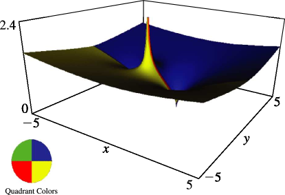
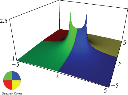
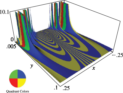
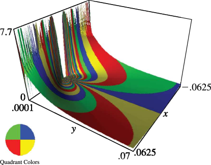
… ►In Figures 23.16.2 and 23.16.3, height corresponds to the absolute value of the function and color to the phase. … ►

►►

Figure 23.16.1: Modular functions $\lambda \left(\mathrm{i}y\right)$, $J\left(\mathrm{i}y\right)$, $\eta \left(\mathrm{i}y\right)$ for $0\le y\le 3$. … Magnify

►

►

►

Figure 23.16.2: Elliptic modular function $\lambda \left(x+\mathrm{i}y\right)$ for $-0.25\le x\le 0.25$, $0.005\le y\le 0.1$. Magnify 3D Help

►

►

►

Figure 23.16.3: Dedekind’s eta function $\eta \left(x+\mathrm{i}y\right)$ for $-0.0625\le x\le 0.0625$, $0.0001\le y\le 0.07$. Magnify 3D Help

39: 13.4 Integral Representations

… ►The contour of integration starts and terminates at a point $\alpha$ on the real axis between $0$ and $1$. …The fractional powers are continuous and assume their principal values at $t=\alpha$. …At the point where the contour crosses the interval $(1,\mathrm{\infty })$, $t^{-b}$ and the ${}_2{}^{}𝐅_1^{}$ function assume their principal values; compare §§15.1 and 15.2(i). …At this point the fractional powers are determined by $\mathrm{ph}t=\pi$ and $\mathrm{ph}\left(1+t\right)=0$. … ►If $a\ne 0,-1,-2,\mathrm{\dots }$, then …

40: 31.7 Relations to Other Functions

… ►

31.7.1 $${}_2{}^{}F_1^{}(\alpha ,\beta ;\gamma ;z)=H\mathrm{\ell }(1,\alpha \beta ;\alpha ,\beta ,\gamma ,\delta ;z)=H\mathrm{\ell }(0,0;\alpha ,\beta ,\gamma ,\alpha +\beta +1-\gamma ;z)=H\mathrm{\ell }(a,a\alpha \beta ;\alpha ,\beta ,\gamma ,\alpha +\beta +1-\gamma ;z).$$

ⓘ

Symbols:

${}_2{}^{}F_1^{}(a,b;c;z)$: $=F(a,b;c;z)$ notation for Gauss’ hypergeometric function, $H\mathrm{\ell }(a,q;\alpha ,\beta ,\gamma ,\delta ;z)$: Heun functions, $z$: complex variable, $\gamma$: real or complex parameter, $\delta$: real or complex parameter, $a$: complex parameter, $\alpha$: real or complex parameter and $\beta$: real or complex parameter

Permalink:

http://dlmf.nist.gov/31.7.E1

Encodings:

pMML, png, TeX

See also:

Annotations for §31.7(i), §31.7 and Ch.31

►Other reductions of $H\mathrm{\ell }$ to a ${}_2{}^{}F_1^{}$, with at least one free parameter, exist iff the pair $(a,p)$ takes one of a finite number of values, where $q=\alpha \beta p$. … ►

31.7.3 $$H\mathrm{\ell }(4,\alpha \beta ;\alpha ,\beta ,\frac{1}{2},\frac{2}{3}(\alpha +\beta );z)={}_2{}^{}F_1^{}(\frac{1}{3}\alpha ,\frac{1}{3}\beta ;\frac{1}{2};1-{(1-z)}^2(1-\frac{1}{4}z)),$$

ⓘ

Symbols:

${}_2{}^{}F_1^{}(a,b;c;z)$: $=F(a,b;c;z)$ notation for Gauss’ hypergeometric function, $H\mathrm{\ell }(a,q;\alpha ,\beta ,\gamma ,\delta ;z)$: Heun functions, $z$: complex variable, $\alpha$: real or complex parameter and $\beta$: real or complex parameter

Permalink:

http://dlmf.nist.gov/31.7.E3

Encodings:

pMML, png, TeX

See also:

Annotations for §31.7(i), §31.7 and Ch.31

… ►With $z={\mathrm{sn}}^2(\zeta ,k)$ and …Similar specializations of formulas in §31.3(ii) yield solutions in the neighborhoods of the singularities $\zeta =K$, $K+\mathrm{i}{K}^{\prime }$, and $\mathrm{i}{K}^{\prime }$, where $K$ and $K^{\prime }$ are related to $k$ as in §19.2(ii).