sums%20or%20differences%20of%20squares

SearchAdvancedHelp

(0.004 seconds)

11—20 of 42 matching pages

11: 3.4 Differentiation

… ►

$$B_{-2}^5=\frac{1}{120}(6-10t-15t^2+20t^3-5t^4),$$

… ►

$$B_{-3}^6=-\frac{1}{720}(12-8t-45t^2+20t^3+15t^4-6t^5),$$

►

$$B_{-2}^6=\frac{1}{60}(9-9t-30t^2+20t^3+5t^4-3t^5),$$

… ►

$$B_2^6=-\frac{1}{60}(9+9t-30t^2-20t^3+5t^4+3t^5),$$

… ►For additional formulas involving values of ${\nabla }^{2}u$ and ${\nabla }^{4}u$ on square, triangular, and cubic grids, see Collatz (1960, Table VI, pp. 542–546). …

12: 26.10 Integer Partitions: Other Restrictions

… ► $p(𝒟k,n)$ denotes the number of partitions of $n$ into parts with difference at least $k$. $p({𝒟}^{\prime }3,n)$ denotes the number of partitions of $n$ into parts with difference at least 3, except that multiples of 3 must differ by at least 6. … ►where the last right-hand side is the sum over $m\ge 0$ of the generating functions for partitions into distinct parts with largest part equal to $m$. … ►where the inner sum is the sum of all positive odd divisors of $t$. … ►where the inner sum is the sum of all positive divisors of $t$ that are in $S$. …

13: 25.12 Polylogarithms

… ►

25.12.7 $${\mathrm{Li}}_2\left({\mathrm{e}}^{\mathrm{i}\theta }\right)=\sum _{n=1}^{\mathrm{\infty }}\frac{\cos \left(n\theta \right)}{n^2}+\mathrm{i}\sum _{n=1}^{\mathrm{\infty }}\frac{\sin \left(n\theta \right)}{n^2}.$$

ⓘ

Symbols:

$\cos z$: cosine function, ${\mathrm{Li}}_2\left(z\right)$: dilogarithm, $\mathrm{e}$: base of natural logarithm, $\mathrm{i}$: imaginary unit, $\sin z$: sine function, $n$: nonnegative integer and $\theta$: phase

Keywords:

infinite series, series representation

Source:

Maximon (2003, (8.7), p. 2813)

Referenced by:

§25.12(i)

Permalink:

http://dlmf.nist.gov/25.12.E7

Encodings:

pMML, png, TeX

See also:

Annotations for §25.12(i), §25.12 and Ch.25

►The cosine series in (25.12.7) has the elementary sum … ►

►►

Figure 25.12.1: Dilogarithm function ${\mathrm{Li}}_2\left(x\right)$, Magnify

►

►

►

Figure 25.12.2: Absolute value of the dilogarithm function $\left|{\mathrm{Li}}_2\left(x+\mathrm{i}y\right)\right|$, $-20\le x\le 20$, $-20\le y\le 20$. … Magnify 3D Help

… ►

25.12.10 $${\mathrm{Li}}_s\left(z\right)=\sum _{n=1}^{\mathrm{\infty }}\frac{z^n}{n^s}.$$

ⓘ

Defines:

${\mathrm{Li}}_s\left(z\right)$: polylogarithm

Symbols:

$n$: nonnegative integer, $s$: complex variable and $z$: complex variable

Keywords:

definition, infinite series, series representation

Source:

Lewin (1981, p. 236)

Referenced by:

(25.14.3)

Permalink:

http://dlmf.nist.gov/25.12.E10

Encodings:

pMML, png, TeX

See also:

Annotations for §25.12(ii), §25.12 and Ch.25

…

14: 2.11 Remainder Terms; Stokes Phenomenon

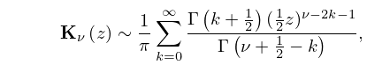
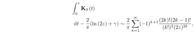
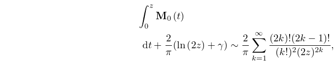
… ►Two different asymptotic expansions in terms of elementary functions, (2.11.6) and (2.11.7), are available for the generalized exponential integral in the sector . … ►We now compute the forward differences ${\mathrm{\Delta }}^j$, $j=0,1,2,\mathrm{\dots }$, of the moduli of the rounded values of the first 6 neglected terms: …Multiplying these differences by ${(-1)}^j{2}^{-j-1}$ and summing, we obtain …Subtraction of this result from the sum of the first 5 terms in (2.11.25) yields 0. … ►For example, using double precision $d_{20}$ is found to agree with (2.11.31) to 13D. …

15: 26.3 Lattice Paths: Binomial Coefficients

… ►

26.3.3 $$\sum _{n=0}^m\left(\genfrac{}{}{0.0pt}{}{m}{n}\right)x^n={(1+x)}^m,$$ $m=0,1,\mathrm{\dots }$,

ⓘ

Symbols:

$\left(\genfrac{}{}{0.0pt}{}{m}{n}\right)$: binomial coefficient, $x$: real variable, $m$: nonnegative integer and $n$: nonnegative integer

A&S Ref:

24.1.1

Permalink:

http://dlmf.nist.gov/26.3.E3

Encodings:

pMML, png, TeX

See also:

Annotations for §26.3(ii), §26.3 and Ch.26

►

26.3.4 $$\sum _{m=0}^{\mathrm{\infty }}\left(\genfrac{}{}{0.0pt}{}{m+n}{m}\right)x^m=\frac{1}{{(1-x)}^{n+1}},$$ .

ⓘ

Symbols:

$\left(\genfrac{}{}{0.0pt}{}{m}{n}\right)$: binomial coefficient, $x$: real variable, $m$: nonnegative integer and $n$: nonnegative integer

A&S Ref:

24.1.1 (in slightly different form)

Permalink:

http://dlmf.nist.gov/26.3.E4

Encodings:

pMML, png, TeX

See also:

Annotations for §26.3(ii), §26.3 and Ch.26

… ►

26.3.7 $$\left(\genfrac{}{}{0.0pt}{}{m+1}{n+1}\right)=\sum _{k=n}^m\left(\genfrac{}{}{0.0pt}{}{k}{n}\right),$$ $m\ge n\ge 0$,

ⓘ

Symbols:

$\left(\genfrac{}{}{0.0pt}{}{m}{n}\right)$: binomial coefficient, $k$: nonnegative integer, $m$: nonnegative integer and $n$: nonnegative integer

Permalink:

http://dlmf.nist.gov/26.3.E7

Encodings:

pMML, png, TeX

See also:

Annotations for §26.3(iii), §26.3 and Ch.26

►

26.3.8 $$\left(\genfrac{}{}{0.0pt}{}{m}{n}\right)=\sum _{k=0}^n\left(\genfrac{}{}{0.0pt}{}{m-n-1+k}{k}\right),$$ $m\ge n\ge 0$.

ⓘ

Symbols:

$\left(\genfrac{}{}{0.0pt}{}{m}{n}\right)$: binomial coefficient, $k$: nonnegative integer, $m$: nonnegative integer and $n$: nonnegative integer

A&S Ref:

24.1.1

Permalink:

http://dlmf.nist.gov/26.3.E8

Encodings:

pMML, png, TeX

See also:

Annotations for §26.3(iii), §26.3 and Ch.26

… ►

26.3.10 $$\left(\genfrac{}{}{0.0pt}{}{m}{n}\right)=\sum _{k=0}^n{(-1)}^{n-k}\left(\genfrac{}{}{0.0pt}{}{m+1}{k}\right),$$ $m\ge n\ge 0$,

ⓘ

Symbols:

$\left(\genfrac{}{}{0.0pt}{}{m}{n}\right)$: binomial coefficient, $k$: nonnegative integer, $m$: nonnegative integer and $n$: nonnegative integer

Permalink:

http://dlmf.nist.gov/26.3.E10

Encodings:

pMML, png, TeX

See also:

Annotations for §26.3(iv), §26.3 and Ch.26

…

16: 26.4 Lattice Paths: Multinomial Coefficients and Set Partitions

… ►

Table 26.4.1: Multinomials and partitions.

► ►►►►

$n$	$m$	$\lambda$	$M_1$	$M_2$	$M_3$
…
$5$	$2$	$2^1,3^1$	$10$	$20$	$10$
$5$	$3$	$1^2,3^1$	$20$	$20$	$10$
…

►

… ►

26.4.9 $${(x_1+x_2+\mathrm{\cdots }+x_k)}^n=\sum \left(\genfrac{}{}{0.0pt}{}{n}{n_1,n_2,\mathrm{\dots },n_k}\right)x_1^{n_1}{x}_2^{n_2}\mathrm{\cdots }{x}_k^{n_k},$$

ⓘ

Symbols:

$\left(\genfrac{}{}{0.0pt}{}{n_1+n_2+\mathrm{\cdots }+n_k}{n_1,n_2,\mathrm{\dots },n_k}\right)$: multinomial coefficient, $x$: real variable, $k$: nonnegative integer and $n$: nonnegative integer

A&S Ref:

24.1.2

Permalink:

http://dlmf.nist.gov/26.4.E9

Encodings:

pMML, png, TeX

See also:

Annotations for §26.4(ii), §26.4 and Ch.26

… ►

26.4.10 $$\left(\genfrac{}{}{0.0pt}{}{n_1+n_2+\mathrm{\cdots }+n_m}{n_1,n_2,\mathrm{\dots },n_m}\right)=\sum _{k=1}^m\left(\genfrac{}{}{0.0pt}{}{n_1+n_2+\mathrm{\cdots }+n_m-1}{n_1,n_2,\mathrm{\dots },n_{k-1},n_k-1,n_{k+1},\mathrm{\dots },n_m}\right),$$ $n_1,n_2,\mathrm{\dots },n_m\ge 1$.

ⓘ

Symbols:

$\left(\genfrac{}{}{0.0pt}{}{n_1+n_2+\mathrm{\cdots }+n_k}{n_1,n_2,\mathrm{\dots },n_k}\right)$: multinomial coefficient, $k$: nonnegative integer, $m$: nonnegative integer and $n$: nonnegative integer

A&S Ref:

24.1.2

Permalink:

http://dlmf.nist.gov/26.4.E10

Encodings:

pMML, png, TeX

See also:

Annotations for §26.4(iii), §26.4 and Ch.26

17: 24.2 Definitions and Generating Functions

… ►

24.2.1 $$\frac{t}{{\mathrm{e}}^t-1}=\sum _{n=0}^{\mathrm{\infty }}{B}_n\frac{t^n}{n!},$$ .

ⓘ

Symbols:

$B_n$: Bernoulli numbers, $\pi$: the ratio of the circumference of a circle to its diameter, $\mathrm{e}$: base of natural logarithm, $!$: factorial (as in $n!$), $n$: integer and $t$: real or complex

Referenced by:

§24.19(ii), §26.14(iii)

Permalink:

http://dlmf.nist.gov/24.2.E1

Encodings:

pMML, png, TeX

See also:

Annotations for §24.2(i), §24.2 and Ch.24

… ►

24.2.5 $$B_n\left(x\right)=\sum _{k=0}^n\left(\genfrac{}{}{0pt}{}{n}{k}\right)B_k{x}^{n-k}.$$

ⓘ

Symbols:

$B_n$: Bernoulli numbers, $B_n\left(x\right)$: Bernoulli polynomials, $\left(\genfrac{}{}{0.0pt}{}{m}{n}\right)$: binomial coefficient, $k$: integer, $n$: integer and $x$: real or complex

Permalink:

http://dlmf.nist.gov/24.2.E5

Encodings:

pMML, png, TeX

See also:

Annotations for §24.2(i), §24.2 and Ch.24

… ►

24.2.10 $$E_n\left(x\right)=\sum _{k=0}^n\left(\genfrac{}{}{0pt}{}{n}{k}\right)\frac{E_k}{2^k}{(x-\frac{1}{2})}^{n-k}.$$

ⓘ

Symbols:

$E_n$: Euler numbers, $E_n\left(x\right)$: Euler polynomials, $\left(\genfrac{}{}{0.0pt}{}{m}{n}\right)$: binomial coefficient, $k$: integer, $n$: integer and $x$: real or complex

A&S Ref:

23.1.7

Permalink:

http://dlmf.nist.gov/24.2.E10

Encodings:

pMML, png, TeX

See also:

Annotations for §24.2(ii), §24.2 and Ch.24

… ►

Table 24.2.5: Coefficients $b_{n,k}$ of the Bernoulli polynomials $B_n\left(x\right)={\sum }_{k=0}^n{b}_{n,k}{x}^k$.

► ►►

	$k$
…

►

►

Table 24.2.6: Coefficients $e_{n,k}$ of the Euler polynomials $E_n\left(x\right)={\sum }_{k=0}^n{e}_{n,k}{x}^k$.

► ►►

	$k$
…

►

18: 11.6 Asymptotic Expansions

… ►

11.6.1 $${𝐊}_{\nu }\left(z\right)\sim \frac{1}{\pi }\sum _{k=0}^{\mathrm{\infty }}\frac{\mathrm{\Gamma }\left(k+\frac{1}{2}\right){(\frac{1}{2}z)}^{\nu -2k-1}}{\mathrm{\Gamma }\left(\nu +\frac{1}{2}-k\right)},$$ $|\mathrm{ph}z|\le \pi -\delta$,

ⓘ

Symbols:

$\mathrm{\Gamma }\left(z\right)$: gamma function, ${𝐊}_{\nu }\left(z\right)$: Struve function, $\sim$: Poincaré asymptotic expansion, $\pi$: the ratio of the circumference of a circle to its diameter, $\mathrm{ph}$: phase, $z$: complex variable, $\nu$: real or complex order, $k$: nonnegative integer and $\delta$: arbitrary small positive constant

A&S Ref:

12.1.29

Referenced by:

§11.6(i), §11.6(i), §11.6(i), §11.6(i)

Permalink:

http://dlmf.nist.gov/11.6.E1

Encodings:

pMML, png, TeX

See also:

Annotations for §11.6(i), §11.6 and Ch.11

… ►

11.6.2 $${𝐌}_{\nu }\left(z\right)\sim \frac{1}{\pi }\sum _{k=0}^{\mathrm{\infty }}{(-1)}^{k+1}\frac{\mathrm{\Gamma }\left(k+\frac{1}{2}\right){(\frac{1}{2}z)}^{\nu -2k-1}}{\mathrm{\Gamma }\left(\nu +\frac{1}{2}-k\right)},$$ $|\mathrm{ph}z|\le \frac{1}{2}\pi -\delta$.

ⓘ

Symbols:

$\mathrm{\Gamma }\left(z\right)$: gamma function, ${𝐌}_{\nu }\left(z\right)$: modified Struve function, $\sim$: Poincaré asymptotic expansion, $\pi$: the ratio of the circumference of a circle to its diameter, $\mathrm{ph}$: phase, $z$: complex variable, $\nu$: real or complex order, $k$: nonnegative integer and $\delta$: arbitrary small positive constant

A&S Ref:

12.2.6

Referenced by:

§11.6(i), §11.6(i), §11.6(i)

Permalink:

http://dlmf.nist.gov/11.6.E2

Encodings:

pMML, png, TeX

See also:

Annotations for §11.6(i), §11.6 and Ch.11

… ►

11.6.3 $${\int }_0^z{𝐊}_0\left(t\right)dt-\frac{2}{\pi }(\ln \left(2z\right)+\gamma )\sim \frac{2}{\pi }\sum _{k=1}^{\mathrm{\infty }}{(-1)}^{k+1}\frac{(2k)!(2k-1)!}{{(k!)}^2{(2z)}^{2k}},$$ $|\mathrm{ph}z|\le \pi -\delta$,

ⓘ

Symbols:

$\gamma$: Euler’s constant, ${𝐊}_{\nu }\left(z\right)$: Struve function, $\sim$: Poincaré asymptotic expansion, $\pi$: the ratio of the circumference of a circle to its diameter, $dx$: differential of $x$ , $!$: factorial (as in $n!$), $\int$: integral, $\ln z$: principal branch of logarithm function, $\mathrm{ph}$: phase, $z$: complex variable, $k$: nonnegative integer and $\delta$: arbitrary small positive constant

A&S Ref:

12.1.32

Referenced by:

§11.6(i)

Permalink:

http://dlmf.nist.gov/11.6.E3

Encodings:

pMML, png, TeX

See also:

Annotations for §11.6(i), §11.6 and Ch.11

►

11.6.4 $${\int }_0^z{𝐌}_0\left(t\right)dt+\frac{2}{\pi }(\ln \left(2z\right)+\gamma )\sim \frac{2}{\pi }\sum _{k=1}^{\mathrm{\infty }}\frac{(2k)!(2k-1)!}{{(k!)}^2{(2z)}^{2k}},$$ $|\mathrm{ph}z|\le \frac{1}{2}\pi -\delta$,

ⓘ

Symbols:

$\gamma$: Euler’s constant, ${𝐌}_{\nu }\left(z\right)$: modified Struve function, $\sim$: Poincaré asymptotic expansion, $\pi$: the ratio of the circumference of a circle to its diameter, $dx$: differential of $x$ , $!$: factorial (as in $n!$), $\int$: integral, $\ln z$: principal branch of logarithm function, $\mathrm{ph}$: phase, $z$: complex variable, $k$: nonnegative integer and $\delta$: arbitrary small positive constant

A&S Ref:

12.2.8

Referenced by:

§11.6(i)

Permalink:

http://dlmf.nist.gov/11.6.E4

Encodings:

pMML, png, TeX

See also:

Annotations for §11.6(i), §11.6 and Ch.11

… ►

$c_3(\lambda )=20{\lambda }^{-6}-4{\lambda }^{-4},$

…

19: 19.36 Methods of Computation

… ►Numerical differences between the variables of a symmetric integral can be reduced in magnitude by successive factors of 4 by repeated applications of the duplication theorem, as shown by (19.26.18). When the differences are moderately small, the iteration is stopped, the elementary symmetric functions of certain differences are calculated, and a polynomial consisting of a fixed number of terms of the sum in (19.19.7) is evaluated. … ►The reductions in §19.29(i) represent $x,y,z$ as squares, for example $x=U_{12}^2$ in (19.29.4). … ►The cases and require different treatment for numerical purposes, and again precautions are needed to avoid cancellations. … ►For computation of Legendre’s integral of the third kind, see Abramowitz and Stegun (1964, §§17.7 and 17.8, Examples 15, 17, 19, and 20). …

20: 18.40 Methods of Computation

… ►Usually, however, other methods are more efficient, especially the numerical solution of difference equations (§3.6) and the application of uniform asymptotic expansions (when available) for OP’s of large degree. … ►

18.40.5 $$F_N(z)=\frac{1}{{\mu }_0}\sum _{n=1}^N\frac{w_n}{z-x_n}.$$

ⓘ

Symbols:

$N$: positive integer, $w_x$: weights, $z$: complex variable, $n$: nonnegative integer and $x$: real variable

Permalink:

http://dlmf.nist.gov/18.40.E5

Encodings:

pMML, png, TeX

See also:

Annotations for §18.40(ii), §18.40(ii), §18.40 and Ch.18

… ►Results of low ($2$ to $3$ decimal digits) precision for $w(x)$ are easily obtained for $N\sim 10$ to $20$. … ►

18.40.7 $${\mu }_N(x)=\sum _{n=1}^N{w}_{n}H\left(x-x_n\right),$$ $x\in (a,b)$,

ⓘ

Symbols:

$H\left(x\right)$: Heaviside function, $\in$: element of, $(a,b)$: open interval, $N$: positive integer, $w_x$: weights, $n$: nonnegative integer and $x$: real variable

Source:

Shohat and Tamarkin (1970, pp. 42-43)

Referenced by:

§18.40(ii)

Permalink:

http://dlmf.nist.gov/18.40.E7

Encodings:

pMML, png, TeX

See also:

Annotations for §18.40(ii), §18.40(ii), §18.40 and Ch.18

…