spherical polar coordinates

SearchAdvancedHelp

(0.001 seconds)

21—30 of 114 matching pages

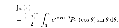
21: 10.54 Integral Representations

§10.54 Integral Representations

… ►

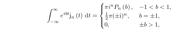
10.54.2 $${𝗃}_n\left(z\right)=\frac{{(-\mathrm{i})}^n}{2}{\int }_0^{\pi }{\mathrm{e}}^{\mathrm{i}z\cos \theta }{P}_n\left(\cos \theta \right)\sin \theta d\theta .$$

ⓘ

Symbols:

$P_n\left(x\right)$: Legendre polynomial, $\pi$: the ratio of the circumference of a circle to its diameter, $\cos z$: cosine function, $dx$: differential of $x$ , $\mathrm{e}$: base of natural logarithm, $\mathrm{i}$: imaginary unit, $\int$: integral, $\sin z$: sine function, ${𝗃}_n\left(z\right)$: spherical Bessel function of the first kind, $n$: integer and $z$: complex variable

A&S Ref:

10.1.14

Permalink:

http://dlmf.nist.gov/10.54.E2

Encodings:

pMML, png, TeX

See also:

Annotations for §10.54 and Ch.10

►

10.54.3 $${𝗄}_n\left(z\right)=\frac{\pi }{2}{\int }_1^{\mathrm{\infty }}{\mathrm{e}}^{-zt}{P}_n\left(t\right)dt,$$

ⓘ

Symbols:

$P_n\left(x\right)$: Legendre polynomial, $\pi$: the ratio of the circumference of a circle to its diameter, $dx$: differential of $x$ , $\mathrm{e}$: base of natural logarithm, $\int$: integral, $\mathrm{ph}$: phase, ${𝗄}_n\left(z\right)$: modified spherical Bessel function, $n$: integer and $z$: complex variable

Permalink:

http://dlmf.nist.gov/10.54.E3

Encodings:

pMML, png, TeX

See also:

Annotations for §10.54 and Ch.10

… ►

${𝗁}_n^{(1)}\left(z\right)={\displaystyle \frac{{(-\mathrm{i})}^{n+1}}{\pi }}{\displaystyle {\int }_{\mathrm{i}\mathrm{\infty }}^{(1+)}}{\mathrm{e}}^{\mathrm{i}zt}{Q}_n\left(t\right)dt,$

… ►For the Legendre polynomial $P_n$ and the associated Legendre function $Q_n$ see §§18.3 and 14.21(i), with $\mu =0$ and $\nu =n$. …

22: 6.10 Other Series Expansions

… ►

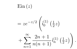
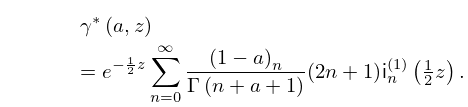
§6.10(ii) Expansions in Series of Spherical Bessel Functions

… ►

6.10.4 $$\mathrm{Si}\left(z\right)=z\sum _{n=0}^{\mathrm{\infty }}{\left({𝗃}_n\left(\frac{1}{2}z\right)\right)}^2,$$

ⓘ

Symbols:

$\mathrm{Si}\left(z\right)$: sine integral, ${𝗃}_n\left(z\right)$: spherical Bessel function of the first kind, $z$: complex variable and $n$: nonnegative integer

Referenced by:

§6.10(ii)

Permalink:

http://dlmf.nist.gov/6.10.E4

Encodings:

pMML, png, TeX

See also:

Annotations for §6.10(ii), §6.10 and Ch.6

►

6.10.5 $$\mathrm{Cin}\left(z\right)=\sum _{n=1}^{\mathrm{\infty }}{a}_n{\left({𝗃}_n\left(\frac{1}{2}z\right)\right)}^2,$$

ⓘ

Symbols:

$\mathrm{Cin}\left(z\right)$: cosine integral, ${𝗃}_n\left(z\right)$: spherical Bessel function of the first kind, $z$: complex variable, $n$: nonnegative integer and $a_n$: coefficients

Permalink:

http://dlmf.nist.gov/6.10.E5

Encodings:

pMML, png, TeX

See also:

Annotations for §6.10(ii), §6.10 and Ch.6

►

6.10.6 $$\mathrm{Ei}\left(x\right)=\gamma +\ln \left|x\right|+\sum _{n=0}^{\mathrm{\infty }}{(-1)}^n(x-a_n){\left({𝗂}_n^{(1)}\left(\frac{1}{2}x\right)\right)}^2,$$ $x\ne 0$,

ⓘ

Symbols:

$\gamma$: Euler’s constant, $\mathrm{Ei}\left(x\right)$: exponential integral, $\ln z$: principal branch of logarithm function, ${𝗂}_n^{(1)}\left(z\right)$: modified spherical Bessel function, $x$: real variable, $n$: nonnegative integer and $a_n$: coefficients

Referenced by:

§6.18(i)

Permalink:

http://dlmf.nist.gov/6.10.E6

Encodings:

pMML, png, TeX

See also:

Annotations for §6.10(ii), §6.10 and Ch.6

… ►

6.10.8 $$\mathrm{Ein}\left(z\right)=z{\mathrm{e}}^{-z/2}\left({𝗂}_0^{(1)}\left(\frac{1}{2}z\right)+\sum _{n=1}^{\mathrm{\infty }}\frac{2n+1}{n(n+1)}{𝗂}_n^{(1)}\left(\frac{1}{2}z\right)\right).$$

ⓘ

Symbols:

$\mathrm{Ein}\left(z\right)$: complementary exponential integral, $\mathrm{e}$: base of natural logarithm, ${𝗂}_n^{(1)}\left(z\right)$: modified spherical Bessel function, $z$: complex variable and $n$: nonnegative integer

Referenced by:

§6.10(ii)

Permalink:

http://dlmf.nist.gov/6.10.E8

Encodings:

pMML, png, TeX

See also:

Annotations for §6.10(ii), §6.10 and Ch.6

…

23: 30.2 Differential Equations

… ►In applications involving prolate spheroidal coordinates ${\gamma }^2$ is positive, in applications involving oblate spheroidal coordinates ${\gamma }^2$ is negative; see §§30.13, 30.14. … ►If $\gamma =0$, Equation (30.2.4) is satisfied by spherical Bessel functions; see (10.47.1).

24: 10.59 Integrals

§10.59 Integrals

►

10.59.1

ⓘ

Symbols:

$P_n\left(x\right)$: Legendre polynomial, $\pi$: the ratio of the circumference of a circle to its diameter, $dx$: differential of $x$ , $\mathrm{e}$: base of natural logarithm, $\mathrm{i}$: imaginary unit, $\int$: integral, ${𝗃}_n\left(z\right)$: spherical Bessel function of the first kind and $n$: integer

A&S Ref:

11.4.26

Referenced by:

§10.59

Permalink:

http://dlmf.nist.gov/10.59.E1

Encodings:

pMML, png, TeX

See also:

Annotations for §10.59 and Ch.10

►where $P_n$ is the Legendre polynomial (§18.3). ►For an integral representation of the Dirac delta in terms of a product of spherical Bessel functions of the first kind see §1.17(ii), and for a generalization see Maximon (1991). …

25: 30.10 Series and Integrals

… ►For expansions in products of spherical Bessel functions, see Flammer (1957, Chapter 6).

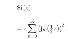
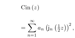
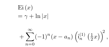
26: 7.6 Series Expansions

… ►

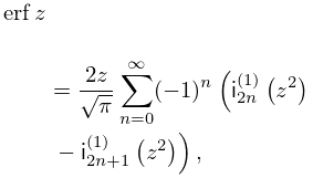
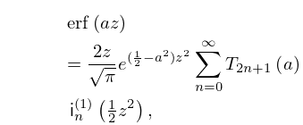
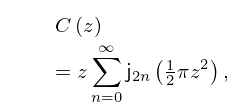
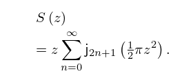
§7.6(ii) Expansions in Series of Spherical Bessel Functions

… ►

7.6.8 $$\mathrm{erf}z=\frac{2z}{\sqrt{\pi }}\sum _{n=0}^{\mathrm{\infty }}{(-1)}^n\left({𝗂}_{2n}^{(1)}\left(z^2\right)-{𝗂}_{2n+1}^{(1)}\left(z^2\right)\right),$$

ⓘ

Symbols:

$\pi$: the ratio of the circumference of a circle to its diameter, $\mathrm{erf}z$: error function, ${𝗂}_n^{(1)}\left(z\right)$: modified spherical Bessel function, $z$: complex variable and $n$: nonnegative integer

A&S Ref:

7.1.7 (in different form)

Referenced by:

§7.6(ii)

Permalink:

http://dlmf.nist.gov/7.6.E8

Encodings:

pMML, png, TeX

See also:

Annotations for §7.6(ii), §7.6 and Ch.7

►

7.6.9 $$\mathrm{erf}\left(az\right)=\frac{2z}{\sqrt{\pi }}{\mathrm{e}}^{(\frac{1}{2}-a^2)z^2}\sum _{n=0}^{\mathrm{\infty }}{T}_{2n+1}\left(a\right){𝗂}_n^{(1)}\left(\frac{1}{2}{z}^2\right),$$ $-1\le a\le 1$.

ⓘ

Symbols:

$T_n\left(x\right)$: Chebyshev polynomial of the first kind, $\pi$: the ratio of the circumference of a circle to its diameter, $\mathrm{erf}z$: error function, $\mathrm{e}$: base of natural logarithm, ${𝗂}_n^{(1)}\left(z\right)$: modified spherical Bessel function, $z$: complex variable and $n$: nonnegative integer

Referenced by:

§7.6(ii)

Permalink:

http://dlmf.nist.gov/7.6.E9

Encodings:

pMML, png, TeX

See also:

Annotations for §7.6(ii), §7.6 and Ch.7

►

7.6.10 $$C\left(z\right)=z\sum _{n=0}^{\mathrm{\infty }}{𝗃}_{2n}\left(\frac{1}{2}\pi z^2\right),$$

ⓘ

Symbols:

$C\left(z\right)$: Fresnel integral, $\pi$: the ratio of the circumference of a circle to its diameter, ${𝗃}_n\left(z\right)$: spherical Bessel function of the first kind, $z$: complex variable and $n$: nonnegative integer

Referenced by:

§7.6(ii)

Permalink:

http://dlmf.nist.gov/7.6.E10

Encodings:

pMML, png, TeX

See also:

Annotations for §7.6(ii), §7.6 and Ch.7

►

7.6.11 $$S\left(z\right)=z\sum _{n=0}^{\mathrm{\infty }}{𝗃}_{2n+1}\left(\frac{1}{2}\pi z^2\right).$$

ⓘ

Symbols:

$S\left(z\right)$: Fresnel integral, $\pi$: the ratio of the circumference of a circle to its diameter, ${𝗃}_n\left(z\right)$: spherical Bessel function of the first kind, $z$: complex variable and $n$: nonnegative integer

Referenced by:

§7.6(ii)

Permalink:

http://dlmf.nist.gov/7.6.E11

Encodings:

pMML, png, TeX

See also:

Annotations for §7.6(ii), §7.6 and Ch.7

…

27: 36.13 Kelvin’s Ship-Wave Pattern

… ►In a reference frame where the ship is at rest we use polar coordinates $r$ and $\varphi$ with $\varphi =0$ in the direction of the velocity of the water relative to the ship. …

28: 3.5 Quadrature

… ►The $p_n(x)$ are the monic Legendre polynomials, that is, the polynomials $P_n\left(x\right)$ (§18.3) scaled so that the coefficient of the highest power of $x$ in their explicit forms is unity. … ►

Table 3.5.17_5: Recurrence coefficients in (3.5.30) and (3.5.30_5) for monic versions $p_n(x)$ and orthonormal versions $q_n(x)$ of the classical orthogonal polynomials.

► ►►►

$p_n(x)$	$q_n(x)$	${\alpha }_n$	${\beta }_n$	$h_0$
…
$\frac{1}{k_n}{P}_n\left(x\right)$	$\frac{1}{\sqrt{h_n}}{P}_n\left(x\right)$	$0$	$\frac{n^2}{4n^2-1}$	$2$
…

►

… ►The steepest descent path is given by $\mathrm{\Im }\left(t-2\sqrt{t}\right)=0$, or in polar coordinates $t=r{\mathrm{e}}^{\mathrm{i}\theta }$ we have $r={\sec }^2\left(\frac{1}{2}\theta \right)$. …

29: 12.17 Physical Applications

§12.17 Physical Applications

… ►in Cartesian coordinates $x,y,z$ of three-dimensional space (§1.5(ii)). By using instead coordinates of the parabolic cylinder $\xi ,\eta ,\zeta$, defined by … ►In a similar manner coordinates of the paraboloid of revolution transform the Helmholtz equation into equations related to the differential equations considered in this chapter. … …

30: 8.7 Series Expansions

§8.7 Series Expansions

►For the functions $e_n(z)$, ${𝗂}_n^{(1)}\left(z\right)$, and $L_n^{(\alpha )}\left(x\right)$ see (8.4.11), §§10.47(ii), and 18.3, respectively. … ►

8.7.5 $${\gamma }^{\ast }(a,z)={\mathrm{e}}^{-\frac{1}{2}z}\sum _{n=0}^{\mathrm{\infty }}\frac{{\left(1-a\right)}_n}{\mathrm{\Gamma }\left(n+a+1\right)}\left(2n+1\right){𝗂}_n^{(1)}\left(\frac{1}{2}z\right).$$

ⓘ

Symbols:

$\mathrm{\Gamma }\left(z\right)$: gamma function, ${\left(a\right)}_n$: Pochhammer’s symbol (or shifted factorial), $\mathrm{e}$: base of natural logarithm, ${\gamma }^{\ast }(a,z)$: incomplete gamma function, ${𝗂}_n^{(1)}\left(z\right)$: modified spherical Bessel function, $z$: complex variable, $a$: parameter and $n$: nonnegative integer

Referenced by:

§8.7

Permalink:

http://dlmf.nist.gov/8.7.E5

Encodings:

pMML, png, TeX

See also:

Annotations for §8.7 and Ch.8

…