special values of the variable

SearchAdvancedHelp

(0.002 seconds)

31—40 of 83 matching pages

31: 25.12 Polylogarithms

… ►Other notations and names for ${\mathrm{Li}}_2\left(z\right)$ include $S_2(z)$ (Kölbig et al. (1970)), Spence function $\mathrm{Sp}(z)$ (’t Hooft and Veltman (1979)), and ${\mathrm{L}}_2(z)$ (Maximon (2003)). … ►

►

►

Figure 25.12.2: Absolute value of the dilogarithm function $\left|{\mathrm{Li}}_2\left(x+\mathrm{i}y\right)\right|$, $-20\le x\le 20$, $-20\le y\le 20$. Principal value. … Magnify 3D Help

… ►For other values of $z$, ${\mathrm{Li}}_s\left(z\right)$ is defined by analytic continuation. … ►The special case $z=1$ is the Riemann zeta function: $\zeta \left(s\right)={\mathrm{Li}}_s\left(1\right)$. …

32: 5.11 Asymptotic Expansions

… ►Wrench (1968) gives exact values of $g_k$ up to $g_{20}$. Spira (1971) corrects errors in Wrench’s results and also supplies exact and 45D values of $g_k$ for $k=21,22,\mathrm{\dots },30$. … ►uniformly for bounded real values of $x$. … ►

5.11.12 $$\frac{\mathrm{\Gamma }\left(z+a\right)}{\mathrm{\Gamma }\left(z+b\right)}\sim z^{a-b},$$

ⓘ

Symbols:

$\mathrm{\Gamma }\left(z\right)$: gamma function, $\sim$: asymptotic equality, $z$: complex variable, $a$: real or complex variable and $b$: real or complex variable

Referenced by:

§5.11(i)

Permalink:

http://dlmf.nist.gov/5.11.E12

Encodings:

pMML, png, TeX

See also:

Annotations for §5.11(iii), §5.11 and Ch.5

►

5.11.13 $$\frac{\mathrm{\Gamma }\left(z+a\right)}{\mathrm{\Gamma }\left(z+b\right)}\sim z^{a-b}\sum _{k=0}^{\mathrm{\infty }}\frac{G_k(a,b)}{z^k},$$

ⓘ

Symbols:

$\mathrm{\Gamma }\left(z\right)$: gamma function, $\sim$: Poincaré asymptotic expansion, $k$: nonnegative integer, $z$: complex variable, $a$: real or complex variable, $b$: real or complex variable and $G_k(a,b)$: coefficients

A&S Ref:

6.1.47

Permalink:

http://dlmf.nist.gov/5.11.E13

Encodings:

pMML, png, TeX

See also:

Annotations for §5.11(iii), §5.11 and Ch.5

…

33: 25.14 Lerch’s Transcendent

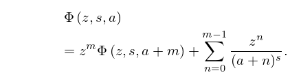
… ►For other values of $z$, $\mathrm{\Phi }(z,s,a)$ is defined by analytic continuation. … ►The Hurwitz zeta function $\zeta (s,a)$ (§25.11) and the polylogarithm ${\mathrm{Li}}_s\left(z\right)$ (§25.12(ii)) are special cases: ►

25.14.2 $$\zeta (s,a)=\mathrm{\Phi }(1,s,a),$$ $\mathrm{\Re }s>1$, $a\ne 0,-1,-2,\mathrm{\dots }$,

ⓘ

Symbols:

$\zeta (s,a)$: Hurwitz zeta function, $\mathrm{\Phi }(z,s,a)$: Lerch’s transcendent, $\mathrm{\Re }$: real part, $a$: real or complex parameter and $s$: complex variable

Keywords:

specialization

Proof sketch:

Derivable from (25.11.1), (25.14.1).

Permalink:

http://dlmf.nist.gov/25.14.E2

Encodings:

pMML, png, TeX

See also:

Annotations for §25.14(i), §25.14 and Ch.25

►

25.14.3 $${\mathrm{Li}}_s\left(z\right)=z\mathrm{\Phi }(z,s,1),$$ $\mathrm{\Re }s>1$, $|z|\le 1$.

ⓘ

Symbols:

$\mathrm{\Phi }(z,s,a)$: Lerch’s transcendent, ${\mathrm{Li}}_s\left(z\right)$: polylogarithm, $\mathrm{\Re }$: real part, $s$: complex variable and $z$: complex variable

Keywords:

specialization

Proof sketch:

Derivable from (25.12.10) and (25.14.1).

Referenced by:

(25.12.12)

Permalink:

http://dlmf.nist.gov/25.14.E3

Encodings:

pMML, png, TeX

See also:

Annotations for §25.14(i), §25.14 and Ch.25

… ►

25.14.4 $$\mathrm{\Phi }(z,s,a)=z^m\mathrm{\Phi }(z,s,a+m)+\sum _{n=0}^{m-1}\frac{z^n}{{(a+n)}^s}.$$

ⓘ

Symbols:

$\mathrm{\Phi }(z,s,a)$: Lerch’s transcendent, $m$: nonnegative integer, $n$: nonnegative integer, $a$: real or complex parameter, $s$: complex variable and $z$: complex variable

Keywords:

recurrence

Source:

Erdélyi et al. (1953a, (1.11.2), p. 27)

Permalink:

http://dlmf.nist.gov/25.14.E4

Encodings:

pMML, png, TeX

See also:

Annotations for §25.14(ii), §25.14 and Ch.25

…

34: 11.10 Anger–Weber Functions

… ►These expansions converge absolutely for all finite values of $z$. … ►

§11.10(vii) Special Values

… ►

11.10.29 $${𝐉}_n\left(z\right)=J_n\left(z\right),$$ $n\in \mathbb{Z}$.

ⓘ

Symbols:

${𝐉}_{\nu }\left(z\right)$: Anger function, $J_{\nu }\left(z\right)$: Bessel function of the first kind, $\in$: element of, $\mathbb{Z}$: set of all integers, $z$: complex variable and $n$: integer order

A&S Ref:

12.3.2

Referenced by:

§11.10(vii), §11.11(ii)

Permalink:

http://dlmf.nist.gov/11.10.E29

Encodings:

pMML, png, TeX

See also:

Annotations for §11.10(vii), §11.10 and Ch.11

… ►

11.10.34 $$2{𝐉}_{\nu }^{\prime }\left(z\right)={𝐉}_{\nu -1}\left(z\right)-{𝐉}_{\nu +1}\left(z\right),$$

ⓘ

Symbols:

${𝐉}_{\nu }\left(z\right)$: Anger function, $z$: complex variable and $\nu$: real or complex order

Permalink:

http://dlmf.nist.gov/11.10.E34

Encodings:

pMML, png, TeX

See also:

Annotations for §11.10(ix), §11.10 and Ch.11

►

11.10.35 $$2{𝐄}_{\nu }^{\prime }\left(z\right)={𝐄}_{\nu -1}\left(z\right)-{𝐄}_{\nu +1}\left(z\right),$$

ⓘ

Symbols:

${𝐄}_{\nu }\left(z\right)$: Weber function, $z$: complex variable and $\nu$: real or complex order

Permalink:

http://dlmf.nist.gov/11.10.E35

Encodings:

pMML, png, TeX

See also:

Annotations for §11.10(ix), §11.10 and Ch.11

…

35: 23.17 Elementary Properties

… ►

§23.17(i) Special Values

… ►

23.17.4 $$\lambda \left(\tau \right)=16q(1-8q+44q^2+\mathrm{\cdots }),$$

ⓘ

Symbols:

$\lambda \left(\tau \right)$: elliptic modular function, $q$: nome and $\tau$: complex variable

Permalink:

http://dlmf.nist.gov/23.17.E4

Encodings:

pMML, png, TeX

See also:

Annotations for §23.17(ii), §23.17 and Ch.23

►

23.17.5 $$1728J\left(\tau \right)=q^{-2}+744+\mathrm{1\hspace{0.33em}96884}{q}^2+\mathrm{214\hspace{0.33em}93760}{q}^4+\mathrm{\cdots },$$

ⓘ

Symbols:

$J\left(\tau \right)$: Klein’s complete invariant, $q$: nome and $\tau$: complex variable

Referenced by:

§23.17(ii)

Permalink:

http://dlmf.nist.gov/23.17.E5

Encodings:

pMML, png, TeX

See also:

Annotations for §23.17(ii), §23.17 and Ch.23

►

23.17.6 $$\eta \left(\tau \right)=\sum _{n=-\mathrm{\infty }}^{\mathrm{\infty }}{(-1)}^n{q}^{{(6n+1)}^2/12}.$$

ⓘ

Symbols:

$\eta \left(\tau \right)$: Dedekind’s eta function (or Dedekind modular function), $q$: nome, $n$: integer and $\tau$: complex variable

Permalink:

http://dlmf.nist.gov/23.17.E6

Encodings:

pMML, png, TeX

See also:

Annotations for §23.17(ii), §23.17 and Ch.23

… ►

23.17.7 $$\lambda \left(\tau \right)=16q\prod _{n=1}^{\mathrm{\infty }}{\left(\frac{1+q^{2n}}{1+q^{2n-1}}\right)}^8,$$

ⓘ

Symbols:

$\lambda \left(\tau \right)$: elliptic modular function, $q$: nome, $n$: integer and $\tau$: complex variable

Permalink:

http://dlmf.nist.gov/23.17.E7

Encodings:

pMML, png, TeX

See also:

Annotations for §23.17(iii), §23.17 and Ch.23

…

36: 8.14 Integrals

… ►

8.14.1 $${\int }_0^{\mathrm{\infty }}{\mathrm{e}}^{-ax}\frac{\gamma (b,x)}{\mathrm{\Gamma }\left(b\right)}dx=\frac{{(1+a)}^{-b}}{a},$$ $\mathrm{\Re }a>0$, $\mathrm{\Re }b>-1$,

ⓘ

Symbols:

$\mathrm{\Gamma }\left(z\right)$: gamma function, $dx$: differential of $x$ , $\mathrm{e}$: base of natural logarithm, $\gamma (a,z)$: incomplete gamma function, $\int$: integral, $\mathrm{\Re }$: real part, $x$: real variable and $a$: parameter

Referenced by:

§8.14, §8.14

Permalink:

http://dlmf.nist.gov/8.14.E1

Encodings:

pMML, png, TeX

See also:

Annotations for §8.14 and Ch.8

►

8.14.2 $${\int }_0^{\mathrm{\infty }}{\mathrm{e}}^{-ax}\mathrm{\Gamma }(b,x)dx=\mathrm{\Gamma }\left(b\right)\frac{1-{(1+a)}^{-b}}{a},$$ $\mathrm{\Re }a>-1$, $\mathrm{\Re }b>-1$.

ⓘ

Symbols:

$\mathrm{\Gamma }\left(z\right)$: gamma function, $dx$: differential of $x$ , $\mathrm{e}$: base of natural logarithm, $\mathrm{\Gamma }(a,z)$: incomplete gamma function, $\int$: integral, $\mathrm{\Re }$: real part, $x$: real variable and $a$: parameter

A&S Ref:

6.5.36

Referenced by:

§8.14, §8.14

Permalink:

http://dlmf.nist.gov/8.14.E2

Encodings:

pMML, png, TeX

See also:

Annotations for §8.14 and Ch.8

►In (8.14.1) and (8.14.2) limiting values are used when $b=0$. ►

8.14.3 $${\int }_0^{\mathrm{\infty }}{x}^{a-1}\gamma (b,x)dx=-\frac{\mathrm{\Gamma }\left(a+b\right)}{a},$$ , $\mathrm{\Re }\left(a+b\right)>0$,

ⓘ

Symbols:

$\mathrm{\Gamma }\left(z\right)$: gamma function, $dx$: differential of $x$ , $\gamma (a,z)$: incomplete gamma function, $\int$: integral, $\mathrm{\Re }$: real part, $x$: real variable and $a$: parameter

Referenced by:

§8.14

Permalink:

http://dlmf.nist.gov/8.14.E3

Encodings:

pMML, png, TeX

See also:

Annotations for §8.14 and Ch.8

►

8.14.4 $${\int }_0^{\mathrm{\infty }}{x}^{a-1}\mathrm{\Gamma }(b,x)dx=\frac{\mathrm{\Gamma }\left(a+b\right)}{a},$$ $\mathrm{\Re }a>0$, $\mathrm{\Re }\left(a+b\right)>0$,

ⓘ

Symbols:

$\mathrm{\Gamma }\left(z\right)$: gamma function, $dx$: differential of $x$ , $\mathrm{\Gamma }(a,z)$: incomplete gamma function, $\int$: integral, $\mathrm{\Re }$: real part, $x$: real variable and $a$: parameter

A&S Ref:

6.5.37

Permalink:

http://dlmf.nist.gov/8.14.E4

Encodings:

pMML, png, TeX

See also:

Annotations for §8.14 and Ch.8

…

37: 18.9 Recurrence Relations and Derivatives

… ►with initial values $p_0(x)=1$ and $p_1(x)=A_{0}x+B_0$. … ►

18.9.2_1 $$x{p}_n(x)=a_n{p}_{n+1}(x)+b_n{p}_n(x)+c_n{p}_{n-1}(x)$$

ⓘ

Symbols:

$p_n(x)$: polynomial of degree $n$ , $n$: nonnegative integer and $x$: real variable

Referenced by:

Table 18.9.2, §18.9(i), Erratum (V1.2.0) Section 18.9

Permalink:

http://dlmf.nist.gov/18.9.E2_1

Encodings:

pMML, png, TeX

See also:

Annotations for §18.9(i), §18.9(i), §18.9 and Ch.18

►with initial values $p_0(x)=1$ and $p_1(x)=a_0^{-1}(x-b_0)$. … ►Formulas (18.9.5), (18.9.11), (18.9.13) are special cases of (18.2.16). Formulas (18.9.6), (18.9.12), (18.9.14) are special cases of (18.2.17). …

38: 2.4 Contour Integrals

… ►Except that $\lambda$ is now permitted to be complex, with $\mathrm{\Re }\lambda >0$, we assume the same conditions on $q(t)$ and also that the Laplace transform in (2.3.8) converges for all sufficiently large values of $\mathrm{\Re }z$. … ►The change of integration variable is given by …By making a further change of variable …and assigning an appropriate value to $c$ to modify the contour, the approximating integral is reducible to an Airy function or a Scorer function (§§9.2, 9.12). … ►The problems sketched in §§2.3(v) and 2.4(v) involve only two of many possibilities for the coalescence of endpoints, saddle points, and singularities in integrals associated with the special functions. …

39: 15.2 Definitions and Analytical Properties

… ►The branch obtained by introducing a cut from $1$ to $+\mathrm{\infty }$ on the real $z$-axis, that is, the branch in the sector $|\mathrm{ph}\left(1-z\right)|\le \pi$, is the principal branch (or principal value) of $F(a,b;c;z)$. ►For all values of $c$ …again with analytic continuation for other values of $z$, and with the principal branch defined in a similar way. … ►Because of the analytic properties with respect to $a$, $b$, and $c$, it is usually legitimate to take limits in formulas involving functions that are undefined for certain values of the parameters. …

40: 29.6 Fourier Series

… ►With $\varphi =\frac{1}{2}\pi -\mathrm{am}(z,k)$, as in (29.2.5), we have ►

29.6.1 $${\mathrm{𝐸𝑐}}_{\nu }^{2m}(z,k^2)=\frac{1}{2}{A}_0+\sum _{p=1}^{\mathrm{\infty }}{A}_{2p}\cos \left(2p\varphi \right).$$

ⓘ

Symbols:

${\mathrm{𝐸𝑐}}_{\nu }^m(z,k^2)$: Lamé function, $\cos z$: cosine function, $m$: nonnegative integer, $p$: nonnegative integer, $z$: complex variable, $k$: real parameter, $\nu$: real parameter, $\varphi$: change of variable and $A_{2p}$: coefficients

Referenced by:

§29.15(i), §29.6(i)

Permalink:

http://dlmf.nist.gov/29.6.E1

Encodings:

pMML, png, TeX

See also:

Annotations for §29.6(i), §29.6 and Ch.29

… ►When $\nu \ne 2n$, where $n$ is a nonnegative integer, it follows from §2.9(i) that for any value of $H$ the system (29.6.4)–(29.6.6) has a unique recessive solution $A_0,A_2,A_4,\mathrm{\dots }$; furthermore … ►In the special case $\nu =2n$, $m=0,1,\mathrm{\dots },n$, there is a unique nontrivial solution with the property $A_{2p}=0$, $p=n+1,n+2,\mathrm{\dots }$. This solution can be constructed from (29.6.4) by backward recursion, starting with $A_{2n+2}=0$ and an arbitrary nonzero value of $A_{2n}$, followed by normalization via (29.6.5) and (29.6.6). …