sigma function

SearchAdvancedHelp

(0.004 seconds)

31—40 of 73 matching pages

31: Bibliography C

… ►

Gauss hypergeometric representations of the Ferrers function of the second kind. SIGMA Symmetry Integrability Geom. Methods Appl. 17, pp. Paper 053, 33.

ⓘ

External Links:

Document, Link, MathReview Entry, ZentralBlatt

Referenced by:

(14.13.2), §14.3(iii), §14.3(iii).

Encodings:

BibTeX

… ►

On parameter differentiation for integral representations of associated Legendre functions. SIGMA Symmetry Integrability Geom. Methods Appl. 7, pp. Paper 050, 16.

ⓘ

External Links:

ISSN 1815-0659, Document, FullText, MathReview (Michael Doschoris), ZentralBlatt

Referenced by:

§14.11, §14.11.

Encodings:

BibTeX

…

32: Bibliography M

… ►

A connection formula for the $q$-confluent hypergeometric function. SIGMA Symmetry Integrability Geom. Methods Appl. 9, pp. Paper 050, 13.

ⓘ

External Links:

ISSN 1815-0659, Document, MathReview (Jeremy Lovejoy), ZentralBlatt

Referenced by:

§17.6(ii), §17.6(ii).

Encodings:

BibTeX

… ►

Zeros of the function $A{i}^{\prime }(z)-\sigma Ai(z)$ . Differential Equations 11, pp. 797–811.

ⓘ

External Links:

ZentralBlatt

Referenced by:

§9.9(i).

Encodings:

BibTeX

…

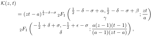
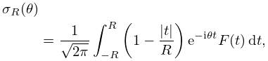
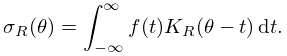
33: 31.10 Integral Equations and Representations

… ►

31.10.9

ⓘ

Symbols:

: Riemann’s $P$-symbol for solutions of the generalized hypergeometric differential equation, $\cos z$: cosine function, $\gamma$: real or complex parameter, $\delta$: real or complex parameter, $ϵ$: real or complex parameter, $\alpha$: real or complex parameter, $\beta$: real or complex parameter, $𝒦(z,t)$: kernel, $\theta$: angle, $\varphi$: angle and $\sigma$: separation constant

Referenced by:

§31.10(i)

Permalink:

http://dlmf.nist.gov/31.10.E9

Encodings:

pMML, png, TeX

See also:

Annotations for §31.10(i), §31.10(i), §31.10 and Ch.31

… ►

31.10.10 $$𝒦(z,t)={(zt-a)}^{\frac{1}{2}-\delta -\sigma }{}_2{}^{}F_1^{}(\genfrac{}{}{0pt}{}{\frac{1}{2}-\delta -\sigma +\alpha ,\frac{1}{2}-\delta -\sigma +\beta }{\gamma };\frac{zt}{a}){}_2{}^{}F_1^{}(\genfrac{}{}{0pt}{}{-\frac{1}{2}+\delta +\sigma ,-\frac{1}{2}+ϵ-\sigma }{\delta };\frac{a(z-1)(t-1)}{(a-1)(zt-a)}),$$

ⓘ

Symbols:

${}_2{}^{}F_1^{}(a,b;c;z)$: $=F(a,b;c;z)$ notation for Gauss’ hypergeometric function, $z$: complex variable, $\gamma$: real or complex parameter, $\delta$: real or complex parameter, $ϵ$: real or complex parameter, $a$: complex parameter, $\alpha$: real or complex parameter, $\beta$: real or complex parameter, $𝒦(z,t)$: kernel and $\sigma$: separation constant

Permalink:

http://dlmf.nist.gov/31.10.E10

Encodings:

pMML, png, TeX

See also:

Annotations for §31.10(i), §31.10(i), §31.10 and Ch.31

… ►

31.10.11

ⓘ

Symbols:

${}_2{}^{}F_1^{}(a,b;c;z)$: $=F(a,b;c;z)$ notation for Gauss’ hypergeometric function, : Riemann’s $P$-symbol for solutions of the generalized hypergeometric differential equation, $z$: complex variable, $\gamma$: real or complex parameter, $\delta$: real or complex parameter, $ϵ$: real or complex parameter, $a$: complex parameter, $\alpha$: real or complex parameter, $\beta$: real or complex parameter, $𝒦(z,t)$: kernel and $\sigma$: separation constant

Permalink:

http://dlmf.nist.gov/31.10.E11

Encodings:

pMML, png, TeX

See also:

Annotations for §31.10(i), §31.10(i), §31.10 and Ch.31

… ►

31.10.19 $$𝒦(u,v,w)=u^{1-\gamma }{v}^{1-\delta }{w}^{1-ϵ}{𝒞}_{1-\gamma }\left(u\sqrt{{\sigma }_1}\right){𝒞}_{1-\delta }\left(v\sqrt{{\sigma }_2}\right){𝒞}_{1-ϵ}\left(\mathrm{i}w\sqrt{{\sigma }_1+{\sigma }_2}\right),$$

ⓘ

Symbols:

${𝒞}_{\nu }\left(z\right)$: cylinder function, $\mathrm{i}$: imaginary unit, $\gamma$: real or complex parameter, $\delta$: real or complex parameter, $ϵ$: real or complex parameter, $𝒦(z;s,t)$: kernel, $u$ , $v$ , $w$ and ${\sigma }_1$, ${\sigma }_2$: separation constants

Permalink:

http://dlmf.nist.gov/31.10.E19

Encodings:

pMML, png, TeX

See also:

Annotations for §31.10(ii), §31.10(ii), §31.10 and Ch.31

…

34: Bibliography L

… ►

More than one third of zeros of Riemann’s zeta-function are on $\sigma =\frac{1}{2}$ . Advances in Math. 13 (4), pp. 383–436.

ⓘ

External Links:

Document, MathReview (H. L. Montgomery), ZentralBlatt

Referenced by:

§25.10(ii), Erratum (V1.1.4) for Subsection 25.10(ii).

Encodings:

BibTeX

…

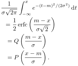
35: 7.20 Mathematical Applications

… ►The normal distribution function with mean $m$ and standard deviation $\sigma$ is given by ►

7.20.1 $$\frac{1}{\sigma \sqrt{2\pi }}{\int }_{-\mathrm{\infty }}^x{\mathrm{e}}^{-{(t-m)}^2/(2{\sigma }^2)}dt=\frac{1}{2}\mathrm{erfc}\left(\frac{m-x}{\sigma \sqrt{2}}\right)=Q\left(\frac{m-x}{\sigma }\right)=P\left(\frac{x-m}{\sigma }\right).$$

ⓘ

Symbols:

$\pi$: the ratio of the circumference of a circle to its diameter, $\mathrm{erfc}z$: complementary error function, $dx$: differential of $x$ , $\mathrm{e}$: base of natural logarithm, $\int$: integral, $x$: real variable, $m$: mean and $\sigma$: standard deviation

A&S Ref:

7.1.22 (slightly modified)

Permalink:

http://dlmf.nist.gov/7.20.E1

Encodings:

pMML, png, TeX

See also:

Annotations for §7.20(iii), §7.20 and Ch.7

…

36: 25.9 Asymptotic Approximations

… ►

25.9.1 $$\zeta \left(\sigma +\mathrm{i}t\right)=\sum _{1\le n\le x}\frac{1}{n^s}+\chi (s)\sum _{1\le n\le y}\frac{1}{n^{1-s}}+O\left(x^{-\sigma }\right)+O\left(y^{\sigma -1}{t}^{\frac{1}{2}-\sigma }\right),$$

ⓘ

Symbols:

$O\left(x\right)$: order not exceeding, $\zeta \left(s\right)$: Riemann zeta function, $\mathrm{i}$: imaginary unit, $n$: nonnegative integer, $x$: real variable, $s$: complex variable and $\sigma$: fixed

Keywords:

asymptotic approximation

Source:

Titchmarsh (1986b, (4.12.4), p. 79)

Referenced by:

§25.9

Permalink:

http://dlmf.nist.gov/25.9.E1

Encodings:

pMML, png, TeX

See also:

Annotations for §25.9 and Ch.25

►where $s=\sigma +\mathrm{i}t$ and …

37: 23.22 Methods of Computation

… ►The functions $\zeta \left(z\right)$ and $\sigma \left(z\right)$ are computed in a similar manner: the former by replacing $u$ and $z$ in (23.6.13) by $z$ and $\pi z/(2{\omega }_1)$, respectively, and also referring to (23.6.8); the latter by applying (23.6.9). …

38: 1.15 Summability Methods

… ►

1.15.44 $${\sigma }_R(\theta )=\frac{1}{\sqrt{2\pi }}{\int }_{-R}^R\left(1-\frac{\left|t\right|}{R}\right){\mathrm{e}}^{-\mathrm{i}\theta t}F(t)dt,$$

ⓘ

Symbols:

$\pi$: the ratio of the circumference of a circle to its diameter, $dx$: differential of $x$ , $\mathrm{e}$: base of natural logarithm, $\mathrm{i}$: imaginary unit, $\int$: integral, $F(x)$: Fourier transform of $f(t)$ , ${\sigma }_R(\theta )$: function and $\left|x\right|$: absolute value of $x$

Permalink:

http://dlmf.nist.gov/1.15.E44

Encodings:

pMML, png, TeX

See also:

Annotations for §1.15(v), §1.15(v), §1.15 and Ch.1

… ►

1.15.45 $${\sigma }_R(\theta )={\int }_{-\mathrm{\infty }}^{\mathrm{\infty }}f(t)K_R(\theta -t)dt.$$

ⓘ

Symbols:

$dx$: differential of $x$ , $\int$: integral, $K_R(s)$: Fejér kernel and ${\sigma }_R(\theta )$: function

Permalink:

http://dlmf.nist.gov/1.15.E45

Encodings:

pMML, png, TeX

See also:

Annotations for §1.15(v), §1.15(v), §1.15 and Ch.1

… ►

1.15.46 $$\underset{R\to \mathrm{\infty }}{lim}{\int }_{-\mathrm{\infty }}^{\mathrm{\infty }}\left|{\sigma }_R(\theta )-f(\theta )\right|d\theta =0.$$

ⓘ

Symbols:

$dx$: differential of $x$ , $\int$: integral, ${\sigma }_R(\theta )$: function and $\left|x\right|$: absolute value of $x$

Permalink:

http://dlmf.nist.gov/1.15.E46

Encodings:

pMML, png, TeX

See also:

Annotations for §1.15(v), §1.15(v), §1.15 and Ch.1

…

39: 2.4 Contour Integrals

… ►

2.4.3 $$q(t)=\frac{1}{2\pi \mathrm{i}}\underset{\eta \to \mathrm{\infty }}{lim}{\int }_{\sigma -\mathrm{i}\eta }^{\sigma +\mathrm{i}\eta }{\mathrm{e}}^{tz}Q(z)dz,$$ ,

ⓘ

Symbols:

$\pi$: the ratio of the circumference of a circle to its diameter, $dx$: differential of $x$ , $\mathrm{e}$: base of natural logarithm, $\mathrm{i}$: imaginary unit, $\int$: integral, $q(t)$: analytic function, $Q(z)$: Laplace transform of $q(t)$ and $\sigma$: constant

Referenced by:

§2.4(ii)

Permalink:

http://dlmf.nist.gov/2.4.E3

Encodings:

pMML, png, TeX

See also:

Annotations for §2.4(ii), §2.4 and Ch.2

… ►

2.4.5 $$q(t)=\frac{1}{2\pi \mathrm{i}}{\int }_{\sigma -\mathrm{i}\mathrm{\infty }}^{\sigma +\mathrm{i}\mathrm{\infty }}{\mathrm{e}}^{tz}Q(z)dz,$$ ,

ⓘ

Symbols:

$\pi$: the ratio of the circumference of a circle to its diameter, $dx$: differential of $x$ , $\mathrm{e}$: base of natural logarithm, $\mathrm{i}$: imaginary unit, $\int$: integral, $q(t)$: analytic function, $Q(z)$: Laplace transform of $q(t)$ and $\sigma$: constant

Permalink:

http://dlmf.nist.gov/2.4.E5

Encodings:

pMML, png, TeX

See also:

Annotations for §2.4(ii), §2.4 and Ch.2

… ►

2.4.6 $$f(t)=\frac{1}{2\pi \mathrm{i}}\underset{\eta \to \mathrm{\infty }}{lim}{\int }_{\sigma -\mathrm{i}\eta }^{\sigma +\mathrm{i}\eta }{\mathrm{e}}^{tz}F(z)dz$$

ⓘ

Symbols:

$\pi$: the ratio of the circumference of a circle to its diameter, $dx$: differential of $x$ , $\mathrm{e}$: base of natural logarithm, $\mathrm{i}$: imaginary unit, $\int$: integral, $\sigma$: constant, $F(z)$: comparison function and $f(x)$: inverse transform of comparison function

Permalink:

http://dlmf.nist.gov/2.4.E6

Encodings:

pMML, png, TeX

See also:

Annotations for §2.4(ii), §2.4 and Ch.2

… ►

2.4.7 $$q(t)-f(t)=\frac{{\mathrm{e}}^{\sigma t}}{2\pi }\underset{\eta \to \mathrm{\infty }}{lim}{\int }_{-\eta }^{\eta }{\mathrm{e}}^{\mathrm{i}t\tau }(Q(\sigma +\mathrm{i}\tau )-F(\sigma +\mathrm{i}\tau ))d\tau .$$

ⓘ

Symbols:

$\pi$: the ratio of the circumference of a circle to its diameter, $dx$: differential of $x$ , $\mathrm{e}$: base of natural logarithm, $\mathrm{i}$: imaginary unit, $\int$: integral, $q(t)$: analytic function, $Q(z)$: Laplace transform of $q(t)$ , $\sigma$: constant, $F(z)$: comparison function and $f(x)$: inverse transform of comparison function

Permalink:

http://dlmf.nist.gov/2.4.E7

Encodings:

pMML, png, TeX

See also:

Annotations for §2.4(ii), §2.4 and Ch.2

…

40: 1.18 Linear Second Order Differential Operators and Eigenfunction Expansions

… ►, $T$ has no eigenfunctions in $L^2\left(X\right)$, then the spectrum $𝝈$ of $T$ consists only of a continuous spectrum, referred to as ${𝝈}_c$. … ►

1.18.52 $$⟨{\left(z-T\right)}^{-1}f,f⟩={\int }_{𝝈}{\left|\widehat{f}(\lambda )\right|}^2\frac{d\lambda }{z-\lambda },$$ $f\in L^2\left(X\right)$, $z\notin {𝝈}_c$,

ⓘ

Symbols:

$L^2(X,dx)$: Lebesgue–Stieltjes measurable, square integrable, complex-valued functions, $dx$: differential of $x$ , $\in$: element of, $⟨f,g⟩$: inner product over functions, $\int$: integral, $\notin$: not an element of, $z$: variable and $\left|x\right|$: absolute value of $x$

Referenced by:

§1.18(vi), §1.18(viii)

Permalink:

http://dlmf.nist.gov/1.18.E52

Encodings:

pMML, png, TeX

See also:

Annotations for §1.18(vi), §1.18(vi), §1.18 and Ch.1

… ►

1.18.64 $$f(x)={\int }_{{𝝈}_c}\widehat{f}(\lambda ){\varphi }_{\lambda }(x)d\lambda +\sum _{{𝝈}_p}\widehat{f}({\lambda }_n){\varphi }_{{\lambda }_n}(x),$$ $f(x)\in C(X)\cap L^2\left(X\right)$.

ⓘ

Symbols:

$L^2(X,dx)$: Lebesgue–Stieltjes measurable, square integrable, complex-valued functions, $dx$: differential of $x$ , $\in$: element of, $\int$: integral, $\cap$: intersection, $C(I)$ or $C(a,b)$: continuous on an interval $I$ or $(a,b)$ and $n$: nonnegative integer

Permalink:

http://dlmf.nist.gov/1.18.E64

Encodings:

pMML, png, TeX

See also:

Annotations for §1.18(viii), §1.18 and Ch.1

… ►

1.18.65 $${\int }_X{\left|f(x)\right|}^{2}dx={\int }_{{𝝈}_c}{\left|\widehat{f}(\lambda )\right|}^{2}d\lambda +\sum _{{𝝈}_p}{\left|\widehat{f}({\lambda }_n)\right|}^2,$$ $f\in L^2\left(X\right)$.

ⓘ

Symbols:

$L^2(X,dx)$: Lebesgue–Stieltjes measurable, square integrable, complex-valued functions, $dx$: differential of $x$ , $\in$: element of, $\int$: integral, $n$: nonnegative integer and $\left|x\right|$: absolute value of $x$

Referenced by:

§1.18(viii)

Permalink:

http://dlmf.nist.gov/1.18.E65

Encodings:

pMML, png, TeX

See also:

Annotations for §1.18(viii), §1.18 and Ch.1

… ►

1.18.66 $$⟨{\left(z-T\right)}^{-1}f,f⟩=\sum _{{𝝈}_p}\frac{{\left|\widehat{f}({\lambda }_n)\right|}^2}{z-{\lambda }_n}+{\int }_{{𝝈}_c}{\left|\widehat{f}(\lambda )\right|}^2\frac{d\lambda }{z-\lambda },$$ $f\in L^2\left(X\right)$, $z\notin 𝝈$.

ⓘ

Symbols:

$L^2(X,dx)$: Lebesgue–Stieltjes measurable, square integrable, complex-valued functions, $dx$: differential of $x$ , $\in$: element of, $⟨f,g⟩$: inner product over functions, $\int$: integral, $\notin$: not an element of, $z$: variable, $n$: nonnegative integer and $\left|x\right|$: absolute value of $x$

Referenced by:

§1.18(viii), §1.18(viii)

Permalink:

http://dlmf.nist.gov/1.18.E66

Encodings:

pMML, png, TeX

See also:

Annotations for §1.18(viii), §1.18 and Ch.1

…