q-Racah%20polynomials

SearchAdvancedHelp

(0.003 seconds)

11—20 of 316 matching pages

11: 3.8 Nonlinear Equations

… ►

§3.8(iv) Zeros of Polynomials

►The polynomial … ►

Example. Wilkinson’s Polynomial

… ►Consider $x=20$ and $j=19$. We have $p^{\prime }(20)=19!$ and $a_{19}=1+2+\mathrm{\cdots }+20=210$. …

12: Bibliography I

… ►

The real roots of Bernoulli polynomials. Ann. Univ. Turku. Ser. A I 37, pp. 1–20.

ⓘ

External Links:

MathReview (D. H. Lehmer), ZentralBlatt

Referenced by:

§24.12(i).

Encodings:

BibTeX

… ►

On polynomials orthogonal with respect to certain Sobolev inner products. J. Approx. Theory 65 (2), pp. 151–175.

ⓘ

External Links:

ISSN 0021-9045, Document, MathReview (R. A. Askey), ZentralBlatt

Referenced by:

§18.36(ii).

Encodings:

BibTeX

… ►

Two families of associated Wilson polynomials. Canad. J. Math. 42 (4), pp. 659–695.

ⓘ

External Links:

ISSN 0008-414X, MathReview (Mizan Rahman), ZentralBlatt

Referenced by:

§18.26(iv).

Encodings:

BibTeX

… ►

Two families of orthogonal polynomials related to Jacobi polynomials. Rocky Mountain J. Math. 21 (1), pp. 359–375.

ⓘ

External Links:

ISSN 0035-7596, MathReview (Joaquin Bustoz), ZentralBlatt

Referenced by:

§18.30(i).

Encodings:

BibTeX

… ►

Classical and Quantum Orthogonal Polynomials in One Variable. Encyclopedia of Mathematics and its Applications, Vol. 98, Cambridge University Press, Cambridge.

ⓘ

External Links:

ISBN 978-0-521-78201-2; 0-521-78201-5, MathReview Entry, ZentralBlatt

Referenced by:

§1.4(v), Profile Mourad E.H. Ismail, Erratum (V1.0.20) for Chapter 18 Orthogonal Polynomials.

Encodings:

BibTeX

…

13: 6.20 Approximations

… ►

Hastings (1955) gives several minimax polynomial and rational approximations for $E_1\left(x\right)+\ln x$, $x{\mathrm{e}}^x{E}_1\left(x\right)$, and the auxiliary functions $\mathrm{f}\left(x\right)$ and $\mathrm{g}\left(x\right)$. These are included in Abramowitz and Stegun (1964, Ch. 5).

►

Cody and Thacher (1968) provides minimax rational approximations for $E_1\left(x\right)$, with accuracies up to 20S.

►

Cody and Thacher (1969) provides minimax rational approximations for $\mathrm{Ei}\left(x\right)$, with accuracies up to 20S.

►

MacLeod (1996b) provides rational approximations for the sine and cosine integrals and for the auxiliary functions $\mathrm{f}$ and $\mathrm{g}$, with accuracies up to 20S.

…

14: 24.18 Physical Applications

§24.18 Physical Applications

►Bernoulli polynomials appear in statistical physics (Ordóñez and Driebe (1996)), in discussions of Casimir forces (Li et al. (1991)), and in a study of quark-gluon plasma (Meisinger et al. (2002)). ►Euler polynomials also appear in statistical physics as well as in semi-classical approximations to quantum probability distributions (Ballentine and McRae (1998)).

15: 7.24 Approximations

… ►

Hastings (1955) gives several minimax polynomial and rational approximations for $\mathrm{erf}x$, $\mathrm{erfc}x$ and the auxiliary functions $\mathrm{f}\left(x\right)$ and $\mathrm{g}\left(x\right)$.

►

Cody (1969) provides minimax rational approximations for $\mathrm{erf}x$ and $\mathrm{erfc}x$. The maximum relative precision is about 20S.

… ►

Cody et al. (1970) gives minimax rational approximations to Dawson’s integral $F\left(x\right)$ (maximum relative precision 20S–22S).

…

16: 32.8 Rational Solutions

… ►where the $Q_n(z)$ are monic polynomials (coefficient of highest power of $z$ is $1$) satisfying … ►Next, let $p_m(z)$ be the polynomials defined by $p_m(z)=0$ for , and … ►where $P_m(z)$ and $Q_m(z)$ are polynomials of degree $m$, with no common zeros. … ►where $P_{j,n-1}(z)$ and $Q_{j,n}(z)$ are polynomials of degrees $n-1$ and $n$, respectively, with no common zeros. … ►where $\lambda$, $\mu$ are constants, and $P_{n-1}(z)$, $Q_n(z)$ are polynomials of degrees $n-1$ and $n$, respectively, with no common zeros. …

17: 25.20 Approximations

… ►

Cody et al. (1971) gives rational approximations for $\zeta \left(s\right)$ in the form of quotients of polynomials or quotients of Chebyshev series. The ranges covered are $0.5\le s\le 5$, $5\le s\le 11$, $11\le s\le 25$, $25\le s\le 55$. Precision is varied, with a maximum of 20S.

…

18: Bibliography K

… ►

Algorithm 737: INTLIB: A portable Fortran 77 interval standard-function library. ACM Trans. Math. Software 20 (4), pp. 447–459.

ⓘ

External Links:

ISSN 0098-3500, Document, GAMS (module 737; package TOMS), ZentralBlatt

Referenced by:

1st item.

Encodings:

BibTeX

… ►

Methods of computing the Riemann zeta-function and some generalizations of it. USSR Comput. Math. and Math. Phys. 20 (6), pp. 212–230.

ⓘ

External Links:

Document, MathReview (Matti Jutila), ZentralBlatt

Referenced by:

§25.18(i).

Encodings:

BibTeX

… ►

Connection formulae for asymptotics of solutions of the degenerate third Painlevé equation. I. Inverse Problems 20 (4), pp. 1165–1206.

ⓘ

External Links:

ISSN 0266-5611, Document, MathReview (Shun Shimomura), ZentralBlatt

Referenced by:

§32.11(iv).

Encodings:

BibTeX

… ►

The Askey scheme as a four-manifold with corners. Ramanujan J. 20 (3), pp. 409–439.

ⓘ

External Links:

ISSN 1382-4090, Document, FullText, MathReview (José Luis López), ZentralBlatt

Referenced by:

§18.26(v), §18.26(v).

Encodings:

BibTeX

… ►

HYP and HYPQ. Mathematica packages for the manipulation of binomial sums and hypergeometric series respectively $q$-binomial sums and basic hypergeometric series. Séminaire Lotharingien de Combinatoire 30, pp. 61–76.

ⓘ

Notes:

Also published in J. Symbolic Comput. (1995), v. 20, no. 5–6, pp. 737–744.

External Links:

Code, Document, MathReview (G. Gasper), ZentralBlatt

Referenced by:

1st item.

Encodings:

BibTeX

…

19: 24.3 Graphs

… ►

►►

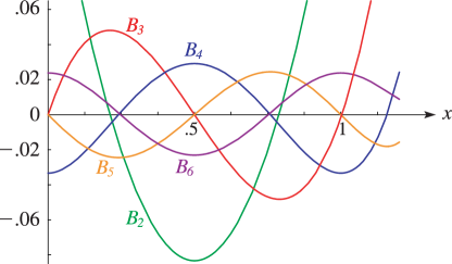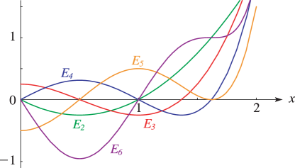Figure 24.3.1: Bernoulli polynomials $B_n\left(x\right)$, $n=2,3,\mathrm{\dots },6$. Magnify

►

►►

Figure 24.3.2: Euler polynomials $E_n\left(x\right)$, $n=2,3,\mathrm{\dots },6$. Magnify

20: 18.4 Graphics

… ►

►►

Figure 18.4.1: Jacobi polynomials $P_n^{(1.5,-0.5)}\left(x\right)$, $n=1,2,3,4,5$. Magnify

►

►►

Figure 18.4.2: Jacobi polynomials $P_n^{(1.25,0.75)}\left(x\right)$, $n=7,8$. … Magnify

… ►

►►

Figure 18.4.4: Legendre polynomials $P_n\left(x\right)$, $n=1,2,3,4,5$. Magnify

►

►►

Figure 18.4.5: Laguerre polynomials $L_n\left(x\right)$, $n=1,2,3,4,5$. Magnify

… ►

►►

Figure 18.4.7: Monic Hermite polynomials $h_n(x)=2^{-n}{H}_n\left(x\right)$, $n=1,2,3,4,5$. Magnify

…