of periodic functions

SearchAdvancedHelp

(0.004 seconds)

21—30 of 70 matching pages

21: 24.17 Mathematical Applications

… ►

24.17.2 $$R_m(n)=\frac{1}{2(m-1)!}{\int }_a^n{f}^{(m)}(x){\tilde{E}}_{m-1}\left(h-x\right)dx.$$

ⓘ

Symbols:

$dx$: differential of $x$ , $!$: factorial (as in $n!$), $\int$: integral, ${\tilde{E}}_n\left(x\right)$: periodic Euler functions, $m$: integer, $x$: real or complex, $h$: parameter, $a$: integer, $n$: integer, $f^{(m)}(x)$: integrable function and $R_m(n)$: remainder

Permalink:

http://dlmf.nist.gov/24.17.E2

Encodings:

pMML, png, TeX

See also:

Annotations for §24.17(i), §24.17(i), §24.17 and Ch.24

… ►

24.17.3 $$S_n(x)=\frac{{\tilde{E}}_n\left(x+\frac{1}{2}n+\frac{1}{2}\right)}{{\tilde{E}}_n\left(\frac{1}{2}n+\frac{1}{2}\right)},$$ $n=0,1,\mathrm{\dots }$,

ⓘ

Symbols:

${\tilde{E}}_n\left(x\right)$: periodic Euler functions, $n$: integer and $x$: real or complex

Permalink:

http://dlmf.nist.gov/24.17.E3

Encodings:

pMML, png, TeX

See also:

Annotations for §24.17(ii), §24.17(ii), §24.17 and Ch.24

… ►

24.17.5

ⓘ

Symbols:

$B_n$: Bernoulli numbers, ${\tilde{B}}_n\left(x\right)$: periodic Bernoulli functions, $n$: integer, $x$: real or complex and $M_n(x)$: function

Permalink:

http://dlmf.nist.gov/24.17.E5

Encodings:

pMML, png, TeX

See also:

Annotations for §24.17(ii), §24.17(ii), §24.17 and Ch.24

… ►

24.17.8 $$F(x)={\tilde{B}}_n\left(x\right)-2^{-n}{B}_n$$

ⓘ

Symbols:

$B_n$: Bernoulli numbers, ${\tilde{B}}_n\left(x\right)$: periodic Bernoulli functions, $n$: integer and $x$: real or complex

Permalink:

http://dlmf.nist.gov/24.17.E8

Encodings:

pMML, png, TeX

See also:

Annotations for §24.17(ii), §24.17(ii), §24.17 and Ch.24

…

22: Bibliography I

… ►

The periodic Lamé functions. Proc. Roy. Soc. Edinburgh 60, pp. 47–63.

ⓘ

External Links:

MathReview (H. Bateman), ZentralBlatt

Referenced by:

§29.1, §29.15(ii), 1st item, §29.7(i).

Encodings:

BibTeX

►

Further investigations into the periodic Lamé functions. Proc. Roy. Soc. Edinburgh 60, pp. 83–99.

ⓘ

External Links:

MathReview (H. Bateman), ZentralBlatt

Referenced by:

§29.1, §29.17(ii), §29.3(iii), §29.6(i), §29.6(ii), §29.6(iii), §29.6(iv), Ch.29, Notations E, Notations E, Notations E, Notations E.

Encodings:

BibTeX

…

23: 1.8 Fourier Series

… ►Formally, if $f(x)$ is a real- or complex-valued $2\pi$-periodic function, … ►Let $f(x)$ be an absolutely integrable function of period $2\pi$, and continuous except at a finite number of points in any bounded interval. … ►If a function $f(x)\in C^2[0,2\pi ]$ is periodic, with period $2\pi$, then the series obtained by differentiating the Fourier series for $f(x)$ term by term converges at every point to $f^{\prime }(x)$. …

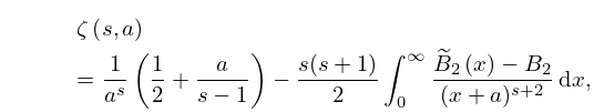
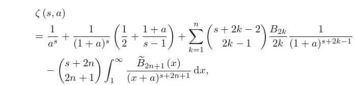
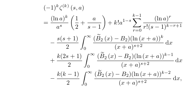
24: 25.11 Hurwitz Zeta Function

… ►

25.11.6 $$\zeta (s,a)=\frac{1}{a^s}\left(\frac{1}{2}+\frac{a}{s-1}\right)-\frac{s(s+1)}{2}{\int }_0^{\mathrm{\infty }}\frac{{\tilde{B}}_2\left(x\right)-B_2}{{(x+a)}^{s+2}}dx,$$ $s\ne 1$, $\mathrm{\Re }s>-1$, $a>0$.

ⓘ

Symbols:

$B_n$: Bernoulli numbers, $\zeta (s,a)$: Hurwitz zeta function, $dx$: differential of $x$ , $\int$: integral, ${\tilde{B}}_n\left(x\right)$: periodic Bernoulli functions, $\mathrm{\Re }$: real part, $x$: real variable, $a$: real or complex parameter and $s$: complex variable

Keywords:

Euler–Maclaurin formula, improper integral

Source:

Apostol (1985a, (25), p. 231)

Referenced by:

Erratum (V1.0.12) for Equations (25.11.6), (25.11.19), and (25.11.20)

Permalink:

http://dlmf.nist.gov/25.11.E6

Encodings:

pMML, png, TeX

Errata (effective with 1.0.12):

Originally the integrand was incorrect because its numerator contained the function ${\tilde{B}}_2\left(x\right)$. The correct function is $\frac{{\tilde{B}}_2\left(x\right)-B_2}{2}$.

Reported 2016-05-08 by Clemens Heuberger

See also:

Annotations for §25.11(iii), §25.11 and Ch.25

►

25.11.7 $$\zeta (s,a)=\frac{1}{a^s}+\frac{1}{{(1+a)}^s}\left(\frac{1}{2}+\frac{1+a}{s-1}\right)+\sum _{k=1}^n\left(\genfrac{}{}{0.0pt}{}{s+2k-2}{2k-1}\right)\frac{B_{2k}}{2k}\frac{1}{{(1+a)}^{s+2k-1}}-\left(\genfrac{}{}{0.0pt}{}{s+2n}{2n+1}\right){\int }_1^{\mathrm{\infty }}\frac{{\tilde{B}}_{2n+1}\left(x\right)}{{(x+a)}^{s+2n+1}}dx,$$ $s\ne 1$, $a>0$, $n=1,2,3,\mathrm{\dots }$, $\mathrm{\Re }s>-2n$.

ⓘ

Symbols:

$B_n$: Bernoulli numbers, $\zeta (s,a)$: Hurwitz zeta function, $\left(\genfrac{}{}{0.0pt}{}{m}{n}\right)$: binomial coefficient, $dx$: differential of $x$ , $\int$: integral, ${\tilde{B}}_n\left(x\right)$: periodic Bernoulli functions, $\mathrm{\Re }$: real part, $k$: nonnegative integer, $n$: nonnegative integer, $x$: real variable, $a$: real or complex parameter and $s$: complex variable

Keywords:

Euler–Maclaurin formula, improper integral

Proof sketch:

Derivable from (25.11.5) by setting $N=1$ and repeatedly integrating by parts using (1.2.6), (24.2.2), (24.2.4), (24.2.11), (24.2.12), (24.4.34).

Permalink:

http://dlmf.nist.gov/25.11.E7

Encodings:

pMML, png, TeX

See also:

Annotations for §25.11(iii), §25.11 and Ch.25

… ►

25.11.19 $${\zeta }^{\prime }(s,a)=-\frac{\ln a}{a^s}\left(\frac{1}{2}+\frac{a}{s-1}\right)-\frac{a^{1-s}}{{(s-1)}^2}+\frac{s(s+1)}{2}{\int }_0^{\mathrm{\infty }}\frac{({\tilde{B}}_2\left(x\right)-B_2)\ln \left(x+a\right)}{{(x+a)}^{s+2}}dx-\frac{(2s+1)}{2}{\int }_0^{\mathrm{\infty }}\frac{{\tilde{B}}_2\left(x\right)-B_2}{{(x+a)}^{s+2}}dx,$$ $\mathrm{\Re }s>-1$, $s\ne 1$, $a>0$.

ⓘ

Symbols:

$B_n$: Bernoulli numbers, $\zeta (s,a)$: Hurwitz zeta function, $dx$: differential of $x$ , $\int$: integral, $\ln z$: principal branch of logarithm function, ${\tilde{B}}_n\left(x\right)$: periodic Bernoulli functions, $\mathrm{\Re }$: real part, $x$: real variable, $a$: real or complex parameter, $s$: complex variable and $k$: integer

Keywords:

derivative

Source:

Apostol (1985a, fourth equation, p. 231); with $k=1$, ${\phi }_2(x)=\frac{1}{2}({\tilde{B}}_2\left(x\right)-B_2)$

Referenced by:

Erratum (V1.0.12) for Equations (25.11.6), (25.11.19), and (25.11.20)

Permalink:

http://dlmf.nist.gov/25.11.E19

Encodings:

pMML, png, TeX

Errata (effective with 1.0.12):

Originally both integrands were incorrect because their numerators contained the function ${\tilde{B}}_2\left(x\right)$. The correct function is $\frac{{\tilde{B}}_2\left(x\right)-B_2}{2}$.

Reported 2016-06-27 by Gergő Nemes

See also:

Annotations for §25.11(vi), §25.11(vi), §25.11 and Ch.25

►

25.11.20 $${(-1)}^k{\zeta }^{(k)}(s,a)=\frac{{(\ln a)}^k}{a^s}\left(\frac{1}{2}+\frac{a}{s-1}\right)+k!a^{1-s}\sum _{r=0}^{k-1}\frac{{(\ln a)}^r}{r!{(s-1)}^{k-r+1}}-\frac{s(s+1)}{2}{\int }_0^{\mathrm{\infty }}\frac{({\tilde{B}}_2\left(x\right)-B_2){(\ln \left(x+a\right))}^k}{{(x+a)}^{s+2}}dx+\frac{k(2s+1)}{2}{\int }_0^{\mathrm{\infty }}\frac{({\tilde{B}}_2\left(x\right)-B_2){(\ln \left(x+a\right))}^{k-1}}{{(x+a)}^{s+2}}dx-\frac{k(k-1)}{2}{\int }_0^{\mathrm{\infty }}\frac{({\tilde{B}}_2\left(x\right)-B_2){(\ln \left(x+a\right))}^{k-2}}{{(x+a)}^{s+2}}dx,$$ $\mathrm{\Re }s>-1$, $s\ne 1$, $a>0$.

ⓘ

Symbols:

$B_n$: Bernoulli numbers, $\zeta (s,a)$: Hurwitz zeta function, $dx$: differential of $x$ , $!$: factorial (as in $n!$), $\int$: integral, $\ln z$: principal branch of logarithm function, ${\tilde{B}}_n\left(x\right)$: periodic Bernoulli functions, $\mathrm{\Re }$: real part, $x$: real variable, $a$: real or complex parameter, $s$: complex variable and $k$: integer

Keywords:

derivative

Source:

Apostol (1985a, fourth equation, p. 231); with ${\phi }_2(x)=\frac{1}{2}({\tilde{B}}_2\left(x\right)-B_2)$

Referenced by:

Erratum (V1.0.12) for Equations (25.11.6), (25.11.19), and (25.11.20)

Permalink:

http://dlmf.nist.gov/25.11.E20

Encodings:

pMML, png, TeX

Errata (effective with 1.0.12):

Originally all three integrands were incorrect because their numerators contained the function ${\tilde{B}}_2\left(x\right)$. The correct function is $\frac{{\tilde{B}}_2\left(x\right)-B_2}{2}$.

Reported 2016-06-27 by Gergő Nemes

See also:

Annotations for §25.11(vi), §25.11(vi), §25.11 and Ch.25

…

25: 4.16 Elementary Properties

… ►

Table 4.16.2: Trigonometric functions: quarter periods and change of sign.

► ►►

$x$	$-\theta$	$\frac{1}{2}\pi \pm \theta$	$\pi \pm \theta$	$\frac{3}{2}\pi \pm \theta$	$2\pi \pm \theta$
…

►

…

26: 28.2 Definitions and Basic Properties

… ►

§28.2(vi) Eigenfunctions

…

27: 24.16 Generalizations

… ►In no particular order, other generalizations include: Bernoulli numbers and polynomials with arbitrary complex index (Butzer et al. (1992)); Euler numbers and polynomials with arbitrary complex index (Butzer et al. (1994)); q-analogs (Carlitz (1954a), Andrews and Foata (1980)); conjugate Bernoulli and Euler polynomials (Hauss (1997, 1998)); Bernoulli–Hurwitz numbers (Katz (1975)); poly-Bernoulli numbers (Kaneko (1997)); Universal Bernoulli numbers (Clarke (1989)); $p$-adic integer order Bernoulli numbers (Adelberg (1996)); $p$-adic $q$-Bernoulli numbers (Kim and Kim (1999)); periodic Bernoulli numbers (Berndt (1975b)); cotangent numbers (Girstmair (1990b)); Bernoulli–Carlitz numbers (Goss (1978)); Bernoulli–Padé numbers (Dilcher (2002)); Bernoulli numbers belonging to periodic functions (Urbanowicz (1988)); cyclotomic Bernoulli numbers (Girstmair (1990a)); modified Bernoulli numbers (Zagier (1998)); higher-order Bernoulli and Euler polynomials with multiple parameters (Erdélyi et al. (1953a, §§1.13.1, 1.14.1)).

28: 22.16 Related Functions

… ►

Quasi-Periodicity

… ►

Quasi-Addition and Quasi-Periodic Formulas

…

29: 29.12 Definitions

… ►In consequence they are doubly-periodic meromorphic functions of $z$. …

30: 20.13 Physical Applications

… ►The functions ${\theta }_j\left(z\right|\tau )$, $j=1,2,3,4$, provide periodic solutions of the partial differential equation … ►Thus the classical theta functions are “periodized”, or “anti-periodized”, Gaussians; see Bellman (1961, pp. 18, 19). …