logarithmic%20integral

SearchAdvancedHelp

(0.003 seconds)

11—20 of 26 matching pages

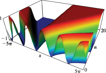
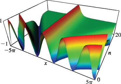
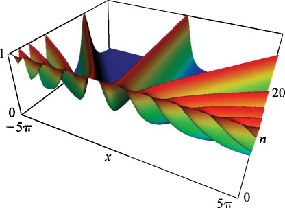
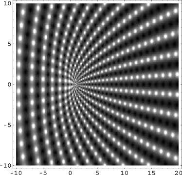
11: 22.3 Graphics

… ►The period diverges logarithmically as $k\to 1-$; see §19.12. ►

►

►

Figure 22.3.13: $\mathrm{sn}(x,k)$ for $k=1-{\mathrm{e}}^{-n}$, $n=0$ to 20, $-5\pi \le x\le 5\pi$. Magnify 3D Help

►

►

►

Figure 22.3.14: $\mathrm{cn}(x,k)$ for $k=1-{\mathrm{e}}^{-n}$, $n=0$ to 20, $-5\pi \le x\le 5\pi$. Magnify 3D Help

►

►

►

Figure 22.3.15: $\mathrm{dn}(x,k)$ for $k=1-{\mathrm{e}}^{-n}$, $n=0$ to 20, $-5\pi \le x\le 5\pi$. Magnify 3D Help

… ►

►►

Figure 22.3.28: Density plot of $|\mathrm{sn}(20,k)|$ as a function of complex $k^2$, $-10\le \mathrm{\Re }\left(k^2\right)\le 20$, $-10\le \mathrm{\Im }\left(k^2\right)\le 10$. … Magnify

…

12: 7.23 Tables

… ►

Abramowitz and Stegun (1964, Chapter 7) includes $\mathrm{erf}x$, $(2/\sqrt{\pi }){\mathrm{e}}^{-x^2}$, $x\in [0,2]$, 10D; $(2/\sqrt{\pi }){\mathrm{e}}^{-x^2}$, $x\in [2,10]$, 8S; $x{\mathrm{e}}^{x^2}\mathrm{erfc}x$, $x^{-2}\in [0,0.25]$, 7D; $2^n\mathrm{\Gamma }\left(\frac{1}{2}n+1\right){\mathrm{i}}^n\mathrm{erfc}\left(x\right)$, $n=1(1)6,10,11$, $x\in [0,5]$, 6S; $F\left(x\right)$, $x\in [0,2]$, 10D; $xF\left(x\right)$, $x^{-2}\in [0,0.25]$, 9D; $C\left(x\right)$, $S\left(x\right)$, $x\in [0,5]$, 7D; $\mathrm{f}\left(x\right)$, $\mathrm{g}\left(x\right)$, $x\in [0,1]$, $x^{-1}\in [0,1]$, 15D.

►

Abramowitz and Stegun (1964, Table 27.6) includes the Goodwin–Staton integral $G\left(x\right)$, $x=1(.1)3(.5)8$, 4D; also $G\left(x\right)+\ln x$, $x=0(.05)1$, 4D.

… ►

Zhang and Jin (1996, pp. 637, 639) includes $(2/\sqrt{\pi }){\mathrm{e}}^{-x^2}$, $\mathrm{erf}x$, $x=0(.02)1(.04)3$, 8D; $C\left(x\right)$, $S\left(x\right)$, $x=0(.2)10(2)100(100)500$, 8D.

… ►

Zhang and Jin (1996, pp. 638, 640–641) includes the real and imaginary parts of $\mathrm{erf}z$, $x\in [0,5]$, $y=0.5(.5)3$, 7D and 8D, respectively; the real and imaginary parts of ${\int }_x^{\mathrm{\infty }}{\mathrm{e}}^{\pm \mathrm{i}{t}^2}dt$, $(1/\sqrt{\pi }){\mathrm{e}}^{\mp \mathrm{i}(x^2+(\pi /4))}{\int }_x^{\mathrm{\infty }}{\mathrm{e}}^{\pm \mathrm{i}{t}^2}dt$, $x=0(.5)20(1)25$, 8D, together with the corresponding modulus and phase to 8D and 6D (degrees), respectively.

… ►

Zhang and Jin (1996, p. 642) includes the first 10 zeros of $\mathrm{erf}z$, 9D; the first 25 distinct zeros of $C\left(z\right)$ and $S\left(z\right)$, 8S.

13: 10.75 Tables

… ►

The main tables in Abramowitz and Stegun (1964, Chapter 9) give $J_0\left(x\right)$ to 15D, $J_1\left(x\right)$, $J_2\left(x\right)$, $Y_0\left(x\right)$, $Y_1\left(x\right)$ to 10D, $Y_2\left(x\right)$ to 8D, $x=0(.1)17.5$; $Y_n\left(x\right)-(2/\pi )J_n\left(x\right)\ln x$, $n=0,1$, $x=0(.1)2$, 8D; $J_n\left(x\right)$, $Y_n\left(x\right)$, $n=3(1)9$, $x=0(.2)20$, 5D or 5S; $J_n\left(x\right)$, $Y_n\left(x\right)$, $n=0(1)20(10)50,100$, $x=1,2,5,10,50,100$, 10S; modulus and phase functions $\sqrt{x}{M}_n\left(x\right)$, ${\theta }_n\left(x\right)-x$, $n=0,1,2$, $1/x=0(.01)0.1$, 8D.

… ►

Zhang and Jin (1996, p. 270) tabulates ${\int }_0^x{J}_0\left(t\right)dt$, ${\int }_0^x{t}^{-1}(1-J_0\left(t\right))dt$, ${\int }_0^x{Y}_0\left(t\right)dt$, ${\int }_x^{\mathrm{\infty }}{t}^{-1}{Y}_0\left(t\right)dt$, $x=0(.1)1(.5)20$, 8D.

… ►

Bickley et al. (1952) tabulates $x^{-n}{I}_n\left(x\right)$ or ${\mathrm{e}}^{-x}{I}_n\left(x\right)$, $x^n{K}_n\left(x\right)$ or ${\mathrm{e}}^x{K}_n\left(x\right)$, $n=2(1)20$, $x=0$(.01 or .1) 10(.1) 20, 8S; $I_n\left(x\right)$, $K_n\left(x\right)$, $n=0(1)20$, $x=0$ or $0.1(.1)20$, 10S.

… ►

The main tables in Abramowitz and Stegun (1964, Chapter 9) give ${\mathrm{e}}^{-x}{I}_n\left(x\right)$, ${\mathrm{e}}^x{K}_n\left(x\right)$, $n=0,1,2$, $x=0(.1)10(.2)20$, 8D–10D or 10S; $\sqrt{x}{\mathrm{e}}^{-x}{I}_n\left(x\right)$, $(\sqrt{x}/\pi )$ ${\mathrm{e}}^x{K}_n\left(x\right)$, $n=0,1,2$, $1/x=0(.002)0.05$; $K_0\left(x\right)+I_0\left(x\right)\ln x$, $x(K_1\left(x\right)-I_1\left(x\right)\ln x)$, $x=0(.1)2$, 8D; ${\mathrm{e}}^{-x}{I}_n\left(x\right)$, ${\mathrm{e}}^x{K}_n\left(x\right)$, $n=3(1)9$, $x=0(.2)10(.5)20$, 5S; $I_n\left(x\right)$, $K_n\left(x\right)$, $n=0(1)20(10)50,100$, $x=1,2,5,10,50,100$, 9–10S.

… ►

Zhang and Jin (1996, p. 271) tabulates ${\mathrm{e}}^{-x}{\int }_0^x{I}_0\left(t\right)dt$, ${\mathrm{e}}^{-x}{\int }_0^x{t}^{-1}(I_0\left(t\right)-1)dt$, ${\mathrm{e}}^x{\int }_x^{\mathrm{\infty }}{K}_0\left(t\right)dt$, $x{\mathrm{e}}^x{\int }_x^{\mathrm{\infty }}{t}^{-1}{K}_0\left(t\right)dt$, $x=0(.1)1(.5)20$, 8D.

…

14: 3.4 Differentiation

… ►If $f$ can be extended analytically into the complex plane, then from Cauchy’s integral formula (§1.9(iii)) …The integral on the right-hand side can be approximated by the composite trapezoidal rule (3.5.2). … ►The integral (3.4.18) becomes …With the choice $r=k$ (which is crucial when $k$ is large because of numerical cancellation) the integrand equals ${\mathrm{e}}^k$ at the dominant points $\theta =0,2\pi$, and in combination with the factor $k^{-k}$ in front of the integral sign this gives a rough approximation to $1/k!$. …As explained in §§3.5(i) and 3.5(ix) the composite trapezoidal rule can be very efficient for computing integrals with analytic periodic integrands. …

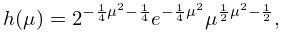
15: 12.10 Uniform Asymptotic Expansions for Large Parameter

… ►

12.10.7 $$\xi =\frac{1}{2}t\sqrt{t^2-1}-\frac{1}{2}\ln \left(t+\sqrt{t^2-1}\right).$$

ⓘ

Defines:

$\xi$ (locally)

Symbols:

$\ln z$: principal branch of logarithm function

Referenced by:

§12.10(vi), §12.10(vii), §12.14(ix)

Permalink:

http://dlmf.nist.gov/12.10.E7

Encodings:

pMML, png, TeX

See also:

Annotations for §12.10(ii), §12.10 and Ch.12

… ►

12.10.15 $$h(\mu )=2^{-\frac{1}{4}{\mu }^2-\frac{1}{4}}{\mathrm{e}}^{-\frac{1}{4}{\mu }^2}{\mu }^{\frac{1}{2}{\mu }^2-\frac{1}{2}},$$

ⓘ

Defines:

$h(\mu )$: expansion (locally)

Symbols:

$\mathrm{e}$: base of natural logarithm

Referenced by:

§12.10(vi)

Permalink:

http://dlmf.nist.gov/12.10.E15

Encodings:

pMML, png, TeX

See also:

Annotations for §12.10(ii), §12.10 and Ch.12

… ►

12.10.26 $$\overline{\xi }=\frac{1}{2}t\sqrt{t^2+1}+\frac{1}{2}\ln \left(t+\sqrt{t^2+1}\right),$$

ⓘ

Defines:

$\overline{\xi }$ (locally)

Symbols:

$\ln z$: principal branch of logarithm function

Permalink:

http://dlmf.nist.gov/12.10.E26

Encodings:

pMML, png, TeX

See also:

Annotations for §12.10(v), §12.10 and Ch.12

… ►

12.10.33 $${𝖠}_{s+1}(\tau )=-4{\tau }^2{(\tau +1)}^2\frac{d}{d\tau }{𝖠}_s(\tau )-\frac{1}{4}{\int }_0^{\tau }\left(20u^2+20u+3\right){𝖠}_s(u)du,$$ $s=0,1,2,\mathrm{\dots }$,

ⓘ

Defines:

${𝖠}_s(\tau )$: coefficients (locally)

Symbols:

$\frac{df}{dx}$: derivative of $f$ with respect to $x$ , $dx$: differential of $x$ , $\int$: integral, $s$: nonnegative integer and $\tau$

Permalink:

http://dlmf.nist.gov/12.10.E33

Encodings:

pMML, png, TeX

See also:

Annotations for §12.10(vi), §12.10 and Ch.12

… ►

$${𝖠}_1(\tau )=-\frac{1}{12}\tau (20{\tau }^2+30\tau +9),$$

…

16: Bibliography K

… ►

Asymptotic approximations for the first incomplete elliptic integral near logarithmic singularity. J. Comput. Appl. Math. 205 (1), pp. 186–206.

ⓘ

External Links:

ISSN 0377-0427, Document, FullText, MathReview (José Luis López), ZentralBlatt

Referenced by:

§19.12, §19.12, §19.36(iv), §19.36(iv).

Encodings:

BibTeX

… ►

Algorithm 737: INTLIB: A portable Fortran 77 interval standard-function library. ACM Trans. Math. Software 20 (4), pp. 447–459.

ⓘ

External Links:

ISSN 0098-3500, Document, GAMS (module 737; package TOMS), ZentralBlatt

Referenced by:

1st item.

Encodings:

BibTeX

… ►

Methods of computing the Riemann zeta-function and some generalizations of it. USSR Comput. Math. and Math. Phys. 20 (6), pp. 212–230.

ⓘ

External Links:

Document, MathReview (Matti Jutila), ZentralBlatt

Referenced by:

§25.18(i).

Encodings:

BibTeX

… ►

Connection formulae for asymptotics of solutions of the degenerate third Painlevé equation. I. Inverse Problems 20 (4), pp. 1165–1206.

ⓘ

External Links:

ISSN 0266-5611, Document, MathReview (Shun Shimomura), ZentralBlatt

Referenced by:

§32.11(iv).

Encodings:

BibTeX

… ►

The Askey scheme as a four-manifold with corners. Ramanujan J. 20 (3), pp. 409–439.

ⓘ

External Links:

ISSN 1382-4090, Document, FullText, MathReview (José Luis López), ZentralBlatt

Referenced by:

§18.26(v), §18.26(v).

Encodings:

BibTeX

…

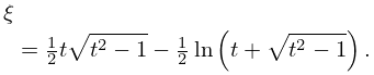
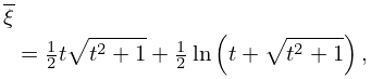
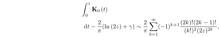
17: 11.6 Asymptotic Expansions

… ►

11.6.3 $${\int }_0^z{𝐊}_0\left(t\right)dt-\frac{2}{\pi }(\ln \left(2z\right)+\gamma )\sim \frac{2}{\pi }\sum _{k=1}^{\mathrm{\infty }}{(-1)}^{k+1}\frac{(2k)!(2k-1)!}{{(k!)}^2{(2z)}^{2k}},$$ $|\mathrm{ph}z|\le \pi -\delta$,

ⓘ

Symbols:

$\gamma$: Euler’s constant, ${𝐊}_{\nu }\left(z\right)$: Struve function, $\sim$: Poincaré asymptotic expansion, $\pi$: the ratio of the circumference of a circle to its diameter, $dx$: differential of $x$ , $!$: factorial (as in $n!$), $\int$: integral, $\ln z$: principal branch of logarithm function, $\mathrm{ph}$: phase, $z$: complex variable, $k$: nonnegative integer and $\delta$: arbitrary small positive constant

A&S Ref:

12.1.32

Referenced by:

§11.6(i)

Permalink:

http://dlmf.nist.gov/11.6.E3

Encodings:

pMML, png, TeX

See also:

Annotations for §11.6(i), §11.6 and Ch.11

►

11.6.4 $${\int }_0^z{𝐌}_0\left(t\right)dt+\frac{2}{\pi }(\ln \left(2z\right)+\gamma )\sim \frac{2}{\pi }\sum _{k=1}^{\mathrm{\infty }}\frac{(2k)!(2k-1)!}{{(k!)}^2{(2z)}^{2k}},$$ $|\mathrm{ph}z|\le \frac{1}{2}\pi -\delta$,

ⓘ

Symbols:

$\gamma$: Euler’s constant, ${𝐌}_{\nu }\left(z\right)$: modified Struve function, $\sim$: Poincaré asymptotic expansion, $\pi$: the ratio of the circumference of a circle to its diameter, $dx$: differential of $x$ , $!$: factorial (as in $n!$), $\int$: integral, $\ln z$: principal branch of logarithm function, $\mathrm{ph}$: phase, $z$: complex variable, $k$: nonnegative integer and $\delta$: arbitrary small positive constant

A&S Ref:

12.2.8

Referenced by:

§11.6(i)

Permalink:

http://dlmf.nist.gov/11.6.E4

Encodings:

pMML, png, TeX

See also:

Annotations for §11.6(i), §11.6 and Ch.11

… ►

11.6.5 $${𝐇}_{\nu }\left(z\right),{𝐋}_{\nu }\left(z\right)\sim \frac{z}{\pi \nu \sqrt{2}}{\left(\frac{\mathrm{e}z}{2\nu }\right)}^{\nu },$$ $|\mathrm{ph}\nu |\le \pi -\delta$.

ⓘ

Symbols:

${𝐇}_{\nu }\left(z\right)$: Struve function, $\sim$: asymptotic equality, $\pi$: the ratio of the circumference of a circle to its diameter, $\mathrm{e}$: base of natural logarithm, ${𝐋}_{\nu }\left(z\right)$: modified Struve function, $\mathrm{ph}$: phase, $z$: complex variable, $\nu$: real or complex order and $\delta$: arbitrary small positive constant

Referenced by:

(11.11.7)

Permalink:

http://dlmf.nist.gov/11.6.E5

Encodings:

pMML, png, TeX

See also:

Annotations for §11.6(ii), §11.6 and Ch.11

… ►

$c_3(\lambda )=20{\lambda }^{-6}-4{\lambda }^{-4},$

…

18: Bibliography

… ►

Exact linearization of a Painlevé transcendent. Phys. Rev. Lett. 38 (20), pp. 1103–1106.

ⓘ

External Links:

Document, MathReview (Mark Adler)

Referenced by:

§32.11(ii), §32.13(i), §32.13(ii), §32.13(iii), §32.5.

Encodings:

BibTeX

… ►

Tables of $\ln \mathrm{\Gamma }(z)$ for Complex Argument. Pergamon Press, New York.

ⓘ

External Links:

ZentralBlatt

Referenced by:

§5.22(iii).

Encodings:

BibTeX

… ►

On the degrees of irreducible factors of higher order Bernoulli polynomials. Acta Arith. 62 (4), pp. 329–342.

ⓘ

External Links:

ISSN 0065-1036, Pdf, MathReview (L. Skula), ZentralBlatt

Referenced by:

§24.12(iii).

Encodings:

BibTeX

… ►

Application of the combined nonlinear-condensation transformation to problems in statistical analysis and theoretical physics. Comput. Phys. Comm. 150 (1), pp. 1–20.

ⓘ

Notes:

Includes algorithms for Lerch’s transcendent. C and Mathematica codes by Aksenov and Jentschura are available.

External Links:

Code, Document

Referenced by:

1st item.

Encodings:

BibTeX

… ►

Repeated integrals and derivatives of $K$ Bessel functions. SIAM J. Math. Anal. 20 (1), pp. 169–175.

ⓘ

External Links:

ISSN 0036-1410, Document, MathReview (A. Haimovici), ZentralBlatt

Referenced by:

§10.43(iii).

Encodings:

BibTeX

…

19: 9.18 Tables

… ►

Miller (1946) tabulates $\mathrm{Ai}\left(x\right)$, ${\mathrm{Ai}}^{\prime }\left(x\right)$ for $x=-20(.01)2;$ ${\log }_{10}\mathrm{Ai}\left(x\right)$, ${\mathrm{Ai}}^{\prime }\left(x\right)/\mathrm{Ai}\left(x\right)$ for $x=0(.1)25(1)75$; $\mathrm{Bi}\left(x\right)$, ${\mathrm{Bi}}^{\prime }\left(x\right)$ for $x=-10(.1)2.5$; ${\log }_{10}\mathrm{Bi}\left(x\right)$, ${\mathrm{Bi}}^{\prime }\left(x\right)/\mathrm{Bi}\left(x\right)$ for $x=0(.1)10$; $M\left(x\right)$, $N\left(x\right)$, $\theta \left(x\right)$, $\varphi \left(x\right)$ (respectively $F(x)$, $G(x)$, $\chi (x)$, $\psi (x)$) for $x=-80(1)-30(.1)0$. Precision is generally 8D; slightly less for some of the auxiliary functions. Extracts from these tables are included in Abramowitz and Stegun (1964, Chapter 10), together with some auxiliary functions for large arguments.

… ►

Zhang and Jin (1996, p. 337) tabulates $\mathrm{Ai}\left(x\right)$, ${\mathrm{Ai}}^{\prime }\left(x\right)$, $\mathrm{Bi}\left(x\right)$, ${\mathrm{Bi}}^{\prime }\left(x\right)$ for $x=0(1)20$ to 8S and for $x=-20(1)0$ to 9D.

… ►

Miller (1946) tabulates $a_k$, ${\mathrm{Ai}}^{\prime }\left(a_k\right)$, $a_k^{\prime }$, $\mathrm{Ai}\left(a_k^{\prime }\right)$, $k=1(1)50$; $b_k$, ${\mathrm{Bi}}^{\prime }\left(b_k\right)$, $b_k^{\prime }$, $\mathrm{Bi}\left(b_k^{\prime }\right)$, $k=1(1)20$. Precision is 8D. Entries for $k=1(1)20$ are reproduced in Abramowitz and Stegun (1964, Chapter 10).

►

Sherry (1959) tabulates $a_k$, ${\mathrm{Ai}}^{\prime }\left(a_k\right)$, $a_k^{\prime }$, $\mathrm{Ai}\left(a_k^{\prime }\right)$, $k=1(1)50$; 20S.

… ►

§9.18(v) Integrals

…

20: 25.6 Integer Arguments

… ►

25.6.3 $$\zeta \left(-n\right)=-\frac{B_{n+1}}{n+1},$$ $n=1,2,3,\mathrm{\dots }$.

ⓘ

Symbols:

$B_n$: Bernoulli numbers, $\zeta \left(s\right)$: Riemann zeta function and $n$: nonnegative integer

Source:

Apostol (1976, (20), p. 266); with $n\ne 0$

A&S Ref:

23.2.15 (in slightly different form)

Permalink:

http://dlmf.nist.gov/25.6.E3

Encodings:

pMML, png, TeX

See also:

Annotations for §25.6(i), §25.6 and Ch.25

… ►

25.6.7 $$\zeta \left(2\right)={\int }_0^1{\int }_0^1\frac{1}{1-xy}dxdy.$$

ⓘ

Symbols:

$\zeta \left(s\right)$: Riemann zeta function, $dx$: differential of $x$ , $\int$: integral and $x$: real variable

Keywords:

double integral

Source:

Apostol (1983, p. 59)

Permalink:

http://dlmf.nist.gov/25.6.E7

Encodings:

pMML, png, TeX

See also:

Annotations for §25.6(i), §25.6 and Ch.25

… ►

25.6.11 $${\zeta }^{\prime }\left(0\right)=-\frac{1}{2}\ln \left(2\pi \right).$$

ⓘ

Symbols:

$\zeta \left(s\right)$: Riemann zeta function, $\pi$: the ratio of the circumference of a circle to its diameter and $\ln z$: principal branch of logarithm function

Source:

Apostol (1985a, p. 223)

A&S Ref:

23.2.13

Permalink:

http://dlmf.nist.gov/25.6.E11

Encodings:

pMML, png, TeX

See also:

Annotations for §25.6(ii), §25.6 and Ch.25

►

25.6.12 $${\zeta }^{\prime \prime }\left(0\right)=-\frac{1}{2}{(\ln \left(2\pi \right))}^2+\frac{1}{2}{\gamma }^2-\frac{1}{24}{\pi }^2+{\gamma }_1,$$

ⓘ

Symbols:

$\gamma$: Euler’s constant, $\zeta \left(s\right)$: Riemann zeta function, ${\gamma }_n$: Stieltjes constants, $\pi$: the ratio of the circumference of a circle to its diameter and $\ln z$: principal branch of logarithm function

Source:

Apostol (1985a, pp. 226, 227, 229)

Referenced by:

Erratum (V1.0.23) for Subsection 25.2(ii) Other Infinite Series

Permalink:

http://dlmf.nist.gov/25.6.E12

Encodings:

pMML, png, TeX

See also:

Annotations for §25.6(ii), §25.6 and Ch.25

… ►

25.6.15 $${\zeta }^{\prime }\left(2n\right)=\frac{{(-1)}^{n+1}{(2\pi )}^{2n}}{2(2n)!}\left(2n{\zeta }^{\prime }\left(1-2n\right)-(\psi \left(2n\right)-\ln \left(2\pi \right))B_{2n}\right).$$

ⓘ

Symbols:

$B_n$: Bernoulli numbers, $\zeta \left(s\right)$: Riemann zeta function, $\pi$: the ratio of the circumference of a circle to its diameter, $\psi \left(z\right)$: psi (or digamma) function, $!$: factorial (as in $n!$), $\ln z$: principal branch of logarithm function and $n$: nonnegative integer

Source:

Miller and Adamchik (1998, (2), p. 202)

Referenced by:

(25.11.21)

Permalink:

http://dlmf.nist.gov/25.6.E15

Encodings:

pMML, png, TeX

See also:

Annotations for §25.6(ii), §25.6 and Ch.25

…