inverse linear

♦ 11—20 of 22 matching pages ♦

(0.001 seconds)

11—20 of 22 matching pages

11: Bibliography S

… ►

D. Shanks (1955) Non-linear transformations of divergent and slowly convergent sequences. J. Math. Phys. 34, pp. 1–42.

ⓘ

External Links:: MathReview (J. Kuntzmann), ZentralBlatt
Referenced by:: §17.18.
Encodings:: BibTeX

… ►

G. E. Shilov (2013) Introduction to the Theory of Linear Spaces. Martino, Mansfield Center, CT.

ⓘ

Notes:: republication of 1961 first edition, Prentice-Hall,New Jersey
External Links:: ISBN 978-1-61427-457-5, MathReview Entry
Referenced by:: §1.18(i), §1.2(vi), §1.3(iv).
Encodings:: BibTeX

… ►

B. D. Sleeman (1969) Non-linear integral equations for Heun functions. Proc. Edinburgh Math. Soc. (2) 16, pp. 281–289.

ⓘ

External Links:: Document, MathReview (J. D. DePree), ZentralBlatt
Referenced by:: §31.10(ii).
Encodings:: BibTeX

… ►

R. Spigler and M. Vianello (1992) Liouville-Green approximations for a class of linear oscillatory difference equations of the second order. J. Comput. Appl. Math. 41 (1-2), pp. 105–116.

ⓘ

External Links:: ISSN 0377-0427, Document, MathReview (Wan Biao Ma), ZentralBlatt
Referenced by:: §2.9(iii).
Encodings:: BibTeX

… ►

R. Spigler (1984) The linear differential equation whose solutions are the products of solutions of two given differential equations. J. Math. Anal. Appl. 98 (1), pp. 130–147.

ⓘ

External Links:: ISSN 0022-247X, Document, FullText, MathReview (Wolfgang Bühring), ZentralBlatt
Referenced by:: §1.13(v).
Encodings:: BibTeX

…

12: Bibliography J

… ►

D. J. Jeffrey, R. M. Corless, D. E. G. Hare, and D. E. Knuth (1995) Sur l’inversion de

y^{\alpha}e^{y}

au moyen des nombres de Stirling associés. C. R. Acad. Sci. Paris Sér. I Math. 320 (12), pp. 1449–1452.

ⓘ

External Links:: ISSN 0764-4442, MathReview (F. Beukers), ZentralBlatt
Referenced by:: (4.13.10).
Encodings:: BibTeX

… ►

M. Jimbo and T. Miwa (1981) Monodromy preserving deformation of linear ordinary differential equations with rational coefficients. II. Phys. D 2 (3), pp. 407–448.

ⓘ

External Links:: ISSN 0167-2789, Document, MathReview (V. A. Golubeva), ZentralBlatt
Referenced by:: §32.4(i), §32.4(ii), §32.4(iv), §32.4(v), §32.6(ii), §32.6(iii), §32.6(iv), §32.6(v), §32.6(v), §32.6(v).
Encodings:: BibTeX

…

13: 15.12 Asymptotic Approximations

… ►

(d)

$\Re z>\tfrac{1}{2}$ and $\alpha_{-}-\tfrac{1}{2}\pi+\delta\leq\operatorname{ph}c\leq\alpha_{+}+\tfrac{1% }{2}\pi-\delta$ , where

15.12.1

\alpha_{\pm}=\operatorname{arctan}\left(\frac{\operatorname{ph}z-\operatorname% {ph}\left(1-z\right)\mp\pi}{\ln|1-z^{-1}|}\right),

ⓘ

Symbols:: $\pi$ : the ratio of the circumference of a circle to its diameter, $\operatorname{arctan}\NVar{z}$ : arctangent function, $\ln\NVar{z}$ : principal branch of logarithm function, $\operatorname{ph}$ : phase, $z$ : complex variable and $\alpha_{\pm}$
Permalink:: http://dlmf.nist.gov/15.12.E1
Encodings:: pMML, png, TeX
See also:: Annotations for §15.12(ii), §15.12 and Ch.15

with $z$ restricted so that $\pm\alpha_{\pm}\in[0,\tfrac{1}{2}\pi)$ .

… ►

15.12.6

\zeta=\operatorname{arccosh}z.

ⓘ

Symbols:: $\operatorname{arccosh}\NVar{z}$ : inverse hyperbolic cosine function, $z$ : complex variable and $\zeta$ : change of variable
Permalink:: http://dlmf.nist.gov/15.12.E6
Encodings:: pMML, png, TeX
See also:: Annotations for §15.12(iii), §15.12 and Ch.15

… ►

15.12.10

\zeta=\operatorname{arccosh}\left(\tfrac{1}{4}z-1\right),

ⓘ

Symbols:: $\operatorname{arccosh}\NVar{z}$ : inverse hyperbolic cosine function, $z$ : complex variable and $\zeta$ : change of variable
Permalink:: http://dlmf.nist.gov/15.12.E10
Encodings:: pMML, png, TeX
See also:: Annotations for §15.12(iii), §15.12 and Ch.15

… ►By combination of the foregoing results of this subsection with the linear transformations of §15.8(i) and the connection formulas of §15.10(ii), similar asymptotic approximations for

F\left(a+e_{1}\lambda,b+e_{2}\lambda;c+e_{3}\lambda;z\right)

can be obtained with

e_{j}=\pm 1

0

j=1,2,3

. …

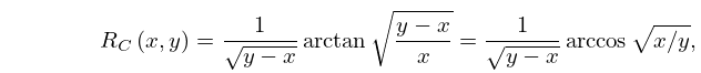
… ►Bulirsch’s integrals are linear combinations of Legendre’s integrals that are chosen to facilitate computational application of Bartky’s transformation (Bartky (1938)). … ►In (19.2.18)–(19.2.22) the inverse trigonometric and hyperbolic functions assume their principal values (§§4.23(ii) and 4.37(ii)). When

x

and

y

are positive,

R_{C}\left(x,y\right)

is an inverse circular function if

x<y

and an inverse hyperbolic function (or logarithm) if

x>y

: ►

19.2.18

R_{C}\left(x,y\right)=\frac{1}{\sqrt{y-x}}\operatorname{arctan}\sqrt{\frac{y-x% }{x}}=\frac{1}{\sqrt{y-x}}\operatorname{arccos}\sqrt{x/y},

0\leq x<y

ⓘ

Symbols:: $R_{C}\left(\NVar{x},\NVar{y}\right)$ : Carlson’s combination of inverse circular and inverse hyperbolic functions, $\operatorname{arccos}\NVar{z}$ : arccosine function and $\operatorname{arctan}\NVar{z}$ : arctangent function
Referenced by:: §19.2(iv)
Permalink:: http://dlmf.nist.gov/19.2.E18
Encodings:: pMML, png, TeX
See also:: Annotations for §19.2(iv), §19.2 and Ch.19

►

19.2.19

R_{C}\left(x,y\right)=\frac{1}{\sqrt{x-y}}\operatorname{arctanh}\sqrt{\frac{x-% y}{x}}=\frac{1}{\sqrt{x-y}}\ln\frac{\sqrt{x}+\sqrt{x-y}}{\sqrt{y}},

0<y<x

ⓘ

Symbols:: $R_{C}\left(\NVar{x},\NVar{y}\right)$ : Carlson’s combination of inverse circular and inverse hyperbolic functions, $\operatorname{arctanh}\NVar{z}$ : inverse hyperbolic tangent function and $\ln\NVar{z}$ : principal branch of logarithm function
Referenced by:: §19.26(i), Figure 19.3.2, Figure 19.3.2, §19.36(ii)
Permalink:: http://dlmf.nist.gov/19.2.E19
Encodings:: pMML, png, TeX
See also:: Annotations for §19.2(iv), §19.2 and Ch.19

…

15: Bibliography R

… ►

M. Rahman (1981) A non-negative representation of the linearization coefficients of the product of Jacobi polynomials. Canad. J. Math. 33 (4), pp. 915–928.

ⓘ

External Links:: ISSN 0008-414X, Document, Link, MathReview (R. A. Askey), ZentralBlatt
Referenced by:: §18.18(v).
Encodings:: BibTeX

… ►

I. S. Reed, D. W. Tufts, X. Yu, T. K. Truong, M. T. Shih, and X. Yin (1990) Fourier analysis and signal processing by use of the Möbius inversion formula. IEEE Trans. Acoustics, Speech, Signal Processing 38, pp. 458–470.

ⓘ

External Links:: ZentralBlatt
Referenced by:: §27.17.
Encodings:: BibTeX

… ►

W. P. Reinhardt (2018) Universality properties of Gaussian quadrature, the derivative rule, and a novel approach to Stieltjes inversion.

ⓘ

Notes:: arXiv:1812.02196
Referenced by:: §18.40(ii).
Encodings:: BibTeX

… ►

E. Ya. Remez (1957) General Computation Methods of Chebyshev Approximation. The Problems with Linear Real Parameters. Publishing House of the Academy of Science of the Ukrainian SSR, Kiev.

ⓘ

Notes:: English translation, AEC-TR-4491, United States Atomic Energy Commission
External Links:: MathReview (A. S. Householder)
Referenced by:: §3.11(iii).
Encodings:: BibTeX

…

16: 24.5 Recurrence Relations

§24.5 Recurrence Relations

… ►

§24.5(iii) Inversion Formulas

…

17: Bibliography K

… ►

A. A. Kapaev (2004) Quasi-linear Stokes phenomenon for the Painlevé first equation. J. Phys. A 37 (46), pp. 11149–11167.

ⓘ

External Links:: ISSN 0305-4470, Document, MathReview (W. Balser), ZentralBlatt
Referenced by:: §32.12(i).
Encodings:: BibTeX

… ►

E. H. Kaufman and T. D. Lenker (1986) Linear convergence and the bisection algorithm. Amer. Math. Monthly 93 (1), pp. 48–51.

ⓘ

External Links:: ISSN 0002-9890, FullText, MathReview (J. G. Herriot), ZentralBlatt
Referenced by:: §3.8(iii).
Encodings:: BibTeX

… ►

V. E. Korepin, N. M. Bogoliubov, and A. G. Izergin (1993) Quantum Inverse Scattering Method and Correlation Functions. Cambridge University Press, Cambridge.

ⓘ

External Links:: ISBN 0-521-37320-4; 0-521-58646-1, MathReview (Makoto Idzumi), ZentralBlatt
Referenced by:: §26.20.
Encodings:: BibTeX

… ►

J. J. Kovacic (1986) An algorithm for solving second order linear homogeneous differential equations. J. Symbolic Comput. 2 (1), pp. 3–43.

ⓘ

External Links:: ISSN 0747-7171, MathReview, ZentralBlatt
Referenced by:: §31.14(ii).
Encodings:: BibTeX

… ►

V. I. Krylov and N. S. Skoblya (1985) A Handbook of Methods of Approximate Fourier Transformation and Inversion of the Laplace Transformation. Mir, Moscow.

ⓘ

Notes:: Translated from the Russian by George Yankovsky. Reprint of the 1977 translation
External Links:: MathReview, ZentralBlatt
Referenced by:: §3.5(viii).
Encodings:: BibTeX

…

18: 3.11 Approximation Techniques

… ►Also, in cases where

f(x)

satisfies a linear ordinary differential equation with polynomial coefficients, the expansion (3.11.11) can be substituted in the differential equation to yield a recurrence relation satisfied by the

c_{n}

. … ►With

b_{0}=1

, the last

q

equations give

b_{1},\dots,b_{q}

as the solution of a system of linear equations. … ►

Laplace Transform Inversion

►Numerical inversion of the Laplace transform (§1.14(iii)) … ►More generally, let

f(x)

be approximated by a linear combination …

19: Bibliography I

… ►

Y. Ikebe, Y. Kikuchi, I. Fujishiro, N. Asai, K. Takanashi, and M. Harada (1993) The eigenvalue problem for infinite compact complex symmetric matrices with application to the numerical computation of complex zeros of

J_{0}(z)-iJ_{1}(z)

and of Bessel functions

J_{m}(z)

of any real order

m

. Linear Algebra Appl. 194, pp. 35–70.

ⓘ

External Links:: ISSN 0024-3795, Document, MathReview (Alan L. Andrew), ZentralBlatt
Referenced by:: §10.21(ix).
Encodings:: BibTeX

… ►

Inverse Symbolic Calculator (website) Centre for Experimental and Constructive Mathematics, Simon Fraser University, Canada.

ⓘ

Notes:: From a decimal approximation, find the most likely exact value.
External Links:: Inverse Symbolic Calculator
Referenced by:: 3rd item.
Encodings:: BibTeX

… ►

A. R. Its and A. A. Kapaev (2003) Quasi-linear Stokes phenomenon for the second Painlevé transcendent. Nonlinearity 16 (1), pp. 363–386.

ⓘ

External Links:: ISSN 0951-7715, Document, MathReview (Youmin Lu), ZentralBlatt
Referenced by:: §32.12(ii).
Encodings:: BibTeX

…

20: 10.21 Zeros

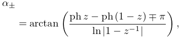
… ►The functions

\rho_{\nu}(t)

and

\sigma_{\nu}(t)

are related to the inverses of the phase functions

\theta_{\nu}\left(x\right)

and

\phi_{\nu}\left(x\right)

defined in §10.18(i): if

\nu\geq 0

, then … ►

\phi_{\nu}\left({y^{\prime}_{\nu,m}}\right)=m\pi,

m=1,2,\dotsc

… ►Next,

z(\zeta)

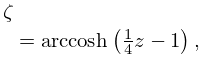
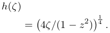
is the inverse of the function

\zeta=\zeta(z)

defined by (10.20.3). … ►

10.21.45

h(\zeta)=\left(4\zeta/(1-z^{2})\right)^{\frac{1}{4}}.

ⓘ

Defines:: $h(\zeta)$ : function (locally)
Symbols:: $z(\zeta)$ : inverse of $\zeta(z)$
A&S Ref:: 9.5.36
Permalink:: http://dlmf.nist.gov/10.21.E45
Encodings:: pMML, png, TeX
See also:: Annotations for §10.21(viii), §10.21 and Ch.10

… ►For describing the distribution of complex zeros by methods based on the Liouville–Green (WKB) approximation for linear homogeneous second-order differential equations, see Segura (2013). …