DLMF: Untitled Document

… ►

§23.3(i) Invariants, Roots, and Discriminant

►The lattice invariants are defined by … ►Given

g_{2}

and

g_{3}

there is a unique lattice

\mathbb{L}

such that (23.3.1) and (23.3.2) are satisfied. …Similarly for

\zeta\left(z;g_{2},g_{3}\right)

and

\sigma\left(z;g_{2},g_{3}\right)

. As functions of

g_{2}

and

g_{3}

,

\wp\left(z;g_{2},g_{3}\right)

and

\zeta\left(z;g_{2},g_{3}\right)

are meromorphic and

\sigma\left(z;g_{2},g_{3}\right)

is entire. …

… ►

See accompanying text — Figure 23.4.1: $\wp\left(x;g_{2},0\right)$ for $0\leq x\leq 9$ , $g_{2}$ = 0. … Magnify

►

…

… ►

23.14.1

\int\wp\left(z\right)\,\mathrm{d}z=-\zeta\left(z\right),

ⓘ

Symbols:: $\wp\left(\NVar{z}\right)$ (= $\wp\left(z|\mathbb{L}\right)$ = $\wp\left(z;g_{2},g_{3}\right)$ ): Weierstrass $\wp$ -function, $\zeta\left(\NVar{z}\right)$ (= $\zeta\left(z|\mathbb{L}\right)$ = $\zeta\left(z;g_{2},g_{3}\right)$ ): Weierstrass zeta function, $\,\mathrm{d}\NVar{x}$ : differential of $x$ , $\int$ : integral, $\mathbb{L}$ : lattice and $z$ : complex
A&S Ref:: 18.6.1
Permalink:: http://dlmf.nist.gov/23.14.E1
Encodings:: pMML, png, TeX
See also:: Annotations for §23.14 and Ch.23

►

23.14.2

\int{\wp}^{2}\left(z\right)\,\mathrm{d}z=\frac{1}{6}\wp'\left(z\right)+\frac{1% }{12}g_{2}z,

ⓘ

Symbols:: $\wp\left(\NVar{z}\right)$ (= $\wp\left(z|\mathbb{L}\right)$ = $\wp\left(z;g_{2},g_{3}\right)$ ): Weierstrass $\wp$ -function, $g_{\NVar{j}}$ : Weierstrass lattice invariants $g_{2}$ , $g_{3}$ , $\,\mathrm{d}\NVar{x}$ : differential of $x$ , $\int$ : integral, $\mathbb{L}$ : lattice and $z$ : complex
A&S Ref:: 18.7.1
Permalink:: http://dlmf.nist.gov/23.14.E2
Encodings:: pMML, png, TeX
See also:: Annotations for §23.14 and Ch.23

►

23.14.3

\int{\wp}^{3}\left(z\right)\,\mathrm{d}z=\frac{1}{120}\wp'''\left(z\right)-% \frac{3}{20}g_{2}\zeta\left(z\right)+\frac{1}{10}g_{3}z.

ⓘ

Symbols:: $\wp\left(\NVar{z}\right)$ (= $\wp\left(z|\mathbb{L}\right)$ = $\wp\left(z;g_{2},g_{3}\right)$ ): Weierstrass $\wp$ -function, $g_{\NVar{j}}$ : Weierstrass lattice invariants $g_{2}$ , $g_{3}$ , $\zeta\left(\NVar{z}\right)$ (= $\zeta\left(z|\mathbb{L}\right)$ = $\zeta\left(z;g_{2},g_{3}\right)$ ): Weierstrass zeta function, $\,\mathrm{d}\NVar{x}$ : differential of $x$ , $\int$ : integral, $\mathbb{L}$ : lattice and $z$ : complex
A&S Ref:: 18.7.2
Permalink:: http://dlmf.nist.gov/23.14.E3
Encodings:: pMML, png, TeX
See also:: Annotations for §23.14 and Ch.23

…

… ►

23.19.2

J\left(\tau\right)=\frac{4}{27}\frac{\left(1-\lambda\left(\tau\right)+{\lambda% }^{2}\left(\tau\right)\right)^{3}}{\left(\lambda\left(\tau\right)\left(1-% \lambda\left(\tau\right)\right)\right)^{2}},

ⓘ

Symbols:: $J\left(\NVar{\tau}\right)$ : Klein’s complete invariant, $\lambda\left(\NVar{\tau}\right)$ : elliptic modular function and $\tau$ : complex variable
Permalink:: http://dlmf.nist.gov/23.19.E2
Encodings:: pMML, png, TeX
See also:: Annotations for §23.19 and Ch.23

►

23.19.3

J\left(\tau\right)=\frac{{g_{2}}^{3}}{{g_{2}}^{3}-27{g_{3}}^{2}},

ⓘ

Symbols:: $J\left(\NVar{\tau}\right)$ : Klein’s complete invariant, $g_{\NVar{j}}$ : Weierstrass lattice invariants $g_{2}$ , $g_{3}$ , $\mathbb{L}$ : lattice and $\tau$ : complex variable
Permalink:: http://dlmf.nist.gov/23.19.E3
Encodings:: pMML, png, TeX
See also:: Annotations for §23.19 and Ch.23

►where

g_{2},g_{3}

are the invariants of the lattice

\mathbb{L}

with generators

1

and

\tau

; see §23.3(i). …

… ►

23.2.4

\wp\left(z\right)=\frac{1}{z^{2}}+\sum_{w\in\mathbb{L}\setminus\{0\}}\left(% \frac{1}{(z-w)^{2}}-\frac{1}{w^{2}}\right),

ⓘ

Defines:: $\wp\left(\NVar{z}\right)$ (= $\wp\left(z|\mathbb{L}\right)$ = $\wp\left(z;g_{2},g_{3}\right)$ ): Weierstrass $\wp$ -function
Symbols:: $\wp\left(\NVar{z};\NVar{g_{2}},\NVar{g_{3}}\right)$ : Weierstrass $\wp$ -function, $g_{\NVar{j}}$ : Weierstrass lattice invariants $g_{2}$ , $g_{3}$ , $\in$ : element of, $\setminus$ : set subtraction, $\mathbb{L}$ : lattice and $z$ : complex
Keywords:: modular functions, Weierstrass $\wp$ -function
Referenced by:: §23.9, Erratum (V1.0.5) for Equation (23.2.4)
Permalink:: http://dlmf.nist.gov/23.2.E4
Encodings:: pMML, png, TeX
Errata (effective with 1.0.5):: Originally the denominator $(z-w)^{2}$ was given incorrectly as $(z-w^{2})$ .
Reported 2012-02-16 by James D. Walker
See also:: Annotations for §23.2(ii), §23.2 and Ch.23

►

23.2.5

\zeta\left(z\right)=\frac{1}{z}+\sum_{w\in\mathbb{L}\setminus\{0\}}\left(\frac% {1}{z-w}+\frac{1}{w}+\frac{z}{w^{2}}\right),

ⓘ

Defines:: $\zeta\left(\NVar{z}\right)$ (= $\zeta\left(z|\mathbb{L}\right)$ = $\zeta\left(z;g_{2},g_{3}\right)$ ): Weierstrass zeta function
Symbols:: $g_{\NVar{j}}$ : Weierstrass lattice invariants $g_{2}$ , $g_{3}$ , $\zeta\left(\NVar{z};\NVar{g_{2}},\NVar{g_{3}}\right)$ : Weierstrass zeta function, $\in$ : element of, $\setminus$ : set subtraction, $\mathbb{L}$ : lattice and $z$ : complex
Keywords:: modular functions, Weierstrass zeta function
Referenced by:: §23.9
Permalink:: http://dlmf.nist.gov/23.2.E5
Encodings:: pMML, png, TeX
See also:: Annotations for §23.2(ii), §23.2 and Ch.23

►

23.2.6

\sigma\left(z\right)=z\prod_{w\in\mathbb{L}\setminus\{0\}}\left(\left(1-\frac{% z}{w}\right)\exp\left(\frac{z}{w}+\frac{z^{2}}{2w^{2}}\right)\right).

ⓘ

Defines:: $\sigma\left(\NVar{z}\right)$ (= $\sigma\left(z|\mathbb{L}\right)$ = $\sigma\left(z;g_{2},g_{3}\right)$ ): Weierstrass sigma function
Symbols:: $g_{\NVar{j}}$ : Weierstrass lattice invariants $g_{2}$ , $g_{3}$ , $\sigma\left(\NVar{z};\NVar{g_{2}},\NVar{g_{3}}\right)$ : Weierstrass sigma function, $\in$ : element of, $\exp\NVar{z}$ : exponential function, $\setminus$ : set subtraction, $\mathbb{L}$ : lattice and $z$ : complex
Keywords:: modular functions, Weierstrass sigma function
Referenced by:: §23.2(iii)
Permalink:: http://dlmf.nist.gov/23.2.E6
Encodings:: pMML, png, TeX
See also:: Annotations for §23.2(ii), §23.2 and Ch.23

… ►

23.2.7

\wp\left(z\right)=-\zeta'\left(z\right),

ⓘ

Symbols:: $\wp\left(\NVar{z}\right)$ (= $\wp\left(z|\mathbb{L}\right)$ = $\wp\left(z;g_{2},g_{3}\right)$ ): Weierstrass $\wp$ -function, $\zeta\left(\NVar{z}\right)$ (= $\zeta\left(z|\mathbb{L}\right)$ = $\zeta\left(z;g_{2},g_{3}\right)$ ): Weierstrass zeta function, $\mathbb{L}$ : lattice and $z$ : complex
A&S Ref:: 18.6.1
Referenced by:: §23.14, §23.3(ii)
Permalink:: http://dlmf.nist.gov/23.2.E7
Encodings:: pMML, png, TeX
See also:: Annotations for §23.2(ii), §23.2 and Ch.23

►

23.2.8

\zeta\left(z\right)=\ifrac{\sigma'\left(z\right)}{\sigma\left(z\right)}.

ⓘ

Symbols:: $\sigma\left(\NVar{z}\right)$ (= $\sigma\left(z|\mathbb{L}\right)$ = $\sigma\left(z;g_{2},g_{3}\right)$ ): Weierstrass sigma function, $\zeta\left(\NVar{z}\right)$ (= $\zeta\left(z|\mathbb{L}\right)$ = $\zeta\left(z;g_{2},g_{3}\right)$ ): Weierstrass zeta function, $\mathbb{L}$ : lattice and $z$ : complex
A&S Ref:: 18.6.2
Referenced by:: §23.3(ii), §23.9
Permalink:: http://dlmf.nist.gov/23.2.E8
Encodings:: pMML, png, TeX
See also:: Annotations for §23.2(ii), §23.2 and Ch.23

…

… ►

23.10.1

\wp\left(u+v\right)=\frac{1}{4}\left(\frac{\wp'\left(u\right)-\wp'\left(v% \right)}{\wp\left(u\right)-\wp\left(v\right)}\right)^{2}-\wp\left(u\right)-\wp% \left(v\right),

ⓘ

Symbols:: $\wp\left(\NVar{z}\right)$ (= $\wp\left(z|\mathbb{L}\right)$ = $\wp\left(z;g_{2},g_{3}\right)$ ): Weierstrass $\wp$ -function and $\mathbb{L}$ : lattice
A&S Ref:: 18.4.1
Referenced by:: §23.10(ii), §23.20(ii), §23.20(ii), §23.23, §23.9
Permalink:: http://dlmf.nist.gov/23.10.E1
Encodings:: pMML, png, TeX
See also:: Annotations for §23.10(i), §23.10 and Ch.23

►

23.10.2

\zeta\left(u+v\right)=\zeta\left(u\right)+\zeta\left(v\right)+\frac{1}{2}\frac% {\zeta''\left(u\right)-\zeta''\left(v\right)}{\zeta'\left(u\right)-\zeta'\left% (v\right)},

ⓘ

Symbols:: $\zeta\left(\NVar{z}\right)$ (= $\zeta\left(z|\mathbb{L}\right)$ = $\zeta\left(z;g_{2},g_{3}\right)$ ): Weierstrass zeta function and $\mathbb{L}$ : lattice
A&S Ref:: 18.4.3
Referenced by:: §23.9
Permalink:: http://dlmf.nist.gov/23.10.E2
Encodings:: pMML, png, TeX
See also:: Annotations for §23.10(i), §23.10 and Ch.23

►

23.10.3

\frac{\sigma\left(u+v\right)\sigma\left(u-v\right)}{{\sigma}^{2}\left(u\right)% {\sigma}^{2}\left(v\right)}=\wp\left(v\right)-\wp\left(u\right),

ⓘ

Symbols:: $\wp\left(\NVar{z}\right)$ (= $\wp\left(z|\mathbb{L}\right)$ = $\wp\left(z;g_{2},g_{3}\right)$ ): Weierstrass $\wp$ -function, $\sigma\left(\NVar{z}\right)$ (= $\sigma\left(z|\mathbb{L}\right)$ = $\sigma\left(z;g_{2},g_{3}\right)$ ): Weierstrass sigma function and $\mathbb{L}$ : lattice
A&S Ref:: 18.4.4
Referenced by:: §23.10(ii)
Permalink:: http://dlmf.nist.gov/23.10.E3
Encodings:: pMML, png, TeX
See also:: Annotations for §23.10(i), §23.10 and Ch.23

… ►

23.10.10

\sigma\left(2z\right)=-\wp'\left(z\right){\sigma}^{4}\left(z\right).

ⓘ

Symbols:: $\wp\left(\NVar{z}\right)$ (= $\wp\left(z|\mathbb{L}\right)$ = $\wp\left(z;g_{2},g_{3}\right)$ ): Weierstrass $\wp$ -function, $\sigma\left(\NVar{z}\right)$ (= $\sigma\left(z|\mathbb{L}\right)$ = $\sigma\left(z;g_{2},g_{3}\right)$ ): Weierstrass sigma function, $\mathbb{L}$ : lattice and $z$ : complex
A&S Ref:: 18.4.8
Referenced by:: §23.10(ii)
Permalink:: http://dlmf.nist.gov/23.10.E10
Encodings:: pMML, png, TeX
See also:: Annotations for §23.10(ii), §23.10 and Ch.23

… ►Also, when

\mathbb{L}

is replaced by

c\mathbb{L}

the lattice invariants

g_{2}

and

g_{3}

are divided by

c^{4}

and

c^{6}

, respectively. …

… ►

23.9.2

\wp\left(z\right)=\frac{1}{z^{2}}+\sum_{n=2}^{\infty}c_{n}z^{2n-2},

0<|z|<|z_{0}|

,

ⓘ

Symbols:: $\wp\left(\NVar{z}\right)$ (= $\wp\left(z|\mathbb{L}\right)$ = $\wp\left(z;g_{2},g_{3}\right)$ ): Weierstrass $\wp$ -function, $\mathbb{L}$ : lattice, $n$ : integer, $z$ : complex and $c_{n}$
A&S Ref:: 18.5.1
Referenced by:: §23.9, §23.9
Permalink:: http://dlmf.nist.gov/23.9.E2
Encodings:: pMML, png, TeX
See also:: Annotations for §23.9 and Ch.23

►

23.9.3

\zeta\left(z\right)=\frac{1}{z}-\sum_{n=2}^{\infty}\frac{c_{n}}{2n-1}z^{2n-1},

0<|z|<|z_{0}|

.

ⓘ

Symbols:: $\zeta\left(\NVar{z}\right)$ (= $\zeta\left(z|\mathbb{L}\right)$ = $\zeta\left(z;g_{2},g_{3}\right)$ ): Weierstrass zeta function, $\mathbb{L}$ : lattice, $n$ : integer, $z$ : complex and $c_{n}$
A&S Ref:: 18.5.5
Referenced by:: §23.9
Permalink:: http://dlmf.nist.gov/23.9.E3
Encodings:: pMML, png, TeX
See also:: Annotations for §23.9 and Ch.23

… ►

c_{2}=\frac{1}{20}g_{2},

►

c_{3}=\frac{1}{28}g_{3},

… ►

23.9.7

\sigma\left(z\right)=\sum_{m,n=0}^{\infty}a_{m,n}(10c_{2})^{m}(56c_{3})^{n}% \frac{z^{4m+6n+1}}{(4m+6n+1)!},

ⓘ

Symbols:: $\sigma\left(\NVar{z}\right)$ (= $\sigma\left(z|\mathbb{L}\right)$ = $\sigma\left(z;g_{2},g_{3}\right)$ ): Weierstrass sigma function, $!$ : factorial (as in $n!$ ), $\mathbb{L}$ : lattice, $n$ : integer, $m$ : integer, $z$ : complex, $c_{n}$ and $a_{m,n}$ : coefficients
A&S Ref:: 18.5.6
Referenced by:: §23.9
Permalink:: http://dlmf.nist.gov/23.9.E7
Encodings:: pMML, png, TeX
See also:: Annotations for §23.9 and Ch.23

…

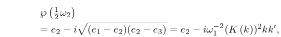
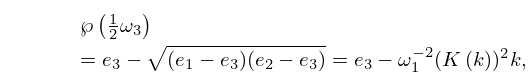
… ►Abramowitz and Stegun (1964) also includes other tables to assist the computation of the Weierstrass functions, for example, the generators as functions of the lattice invariants

g_{2}

and

g_{3}

. …

… ►

23.7.1

\wp\left(\tfrac{1}{2}\omega_{1}\right)=e_{1}+\sqrt{(e_{1}-e_{3})(e_{1}-e_{2})}% =e_{1}+\omega_{1}^{-2}(K\left(k\right))^{2}k^{\prime},

ⓘ

Symbols:: $\wp\left(\NVar{z}\right)$ (= $\wp\left(z|\mathbb{L}\right)$ = $\wp\left(z;g_{2},g_{3}\right)$ ): Weierstrass $\wp$ -function, $e_{\NVar{j}}$ : Weierstrass lattice roots, $K\left(\NVar{k}\right)$ : Legendre’s complete elliptic integral of the first kind, $\mathbb{L}$ : lattice, $\omega_{1}$ , $\omega_{3}$ , $\omega_{2}=-\omega_{1}-\omega_{3}$ : lattice generators, $k$ : modulus and $k^{\prime}$ : complementary modulus
A&S Ref:: 18.3.18
Permalink:: http://dlmf.nist.gov/23.7.E1
Encodings:: pMML, png, TeX
See also:: Annotations for §23.7 and Ch.23

►

23.7.2

\wp\left(\tfrac{1}{2}\omega_{2}\right)=e_{2}-i\sqrt{(e_{1}-e_{2})(e_{2}-e_{3})% }=e_{2}-i\omega_{1}^{-2}(K\left(k\right))^{2}kk^{\prime},

ⓘ

Symbols:: $\wp\left(\NVar{z}\right)$ (= $\wp\left(z|\mathbb{L}\right)$ = $\wp\left(z;g_{2},g_{3}\right)$ ): Weierstrass $\wp$ -function, $e_{\NVar{j}}$ : Weierstrass lattice roots, $K\left(\NVar{k}\right)$ : Legendre’s complete elliptic integral of the first kind, $\mathrm{i}$ : imaginary unit, $\mathbb{L}$ : lattice, $\omega_{1}$ , $\omega_{3}$ , $\omega_{2}=-\omega_{1}-\omega_{3}$ : lattice generators, $k$ : modulus and $k^{\prime}$ : complementary modulus
A&S Ref:: 18.3.18
Permalink:: http://dlmf.nist.gov/23.7.E2
Encodings:: pMML, png, TeX
See also:: Annotations for §23.7 and Ch.23

►

23.7.3

\wp\left(\tfrac{1}{2}\omega_{3}\right)=e_{3}-\sqrt{(e_{1}-e_{3})(e_{2}-e_{3})}% =e_{3}-\omega_{1}^{-2}(K\left(k\right))^{2}k,

ⓘ

Symbols:: $\wp\left(\NVar{z}\right)$ (= $\wp\left(z|\mathbb{L}\right)$ = $\wp\left(z;g_{2},g_{3}\right)$ ): Weierstrass $\wp$ -function, $e_{\NVar{j}}$ : Weierstrass lattice roots, $K\left(\NVar{k}\right)$ : Legendre’s complete elliptic integral of the first kind, $\mathbb{L}$ : lattice, $\omega_{1}$ , $\omega_{3}$ , $\omega_{2}=-\omega_{1}-\omega_{3}$ : lattice generators and $k$ : modulus
A&S Ref:: 18.3.18
Permalink:: http://dlmf.nist.gov/23.7.E3
Encodings:: pMML, png, TeX
See also:: Annotations for §23.7 and Ch.23

…

… ► ►►►

$\mathbb{L}$	lattice in $\mathbb{C}$ .
…
$\Delta$	discriminant ${g_{2}}^{3}-27{g_{3}}^{2}$ .
…

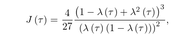
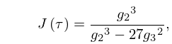
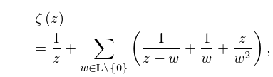
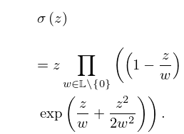
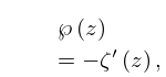
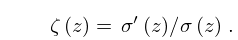
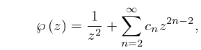
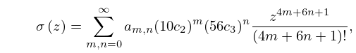
►The main functions treated in this chapter are the Weierstrass

\wp

-function

\wp\left(z\right)=\wp\left(z|\mathbb{L}\right)=\wp\left(z;g_{2},g_{3}\right)

; the Weierstrass zeta function

\zeta\left(z\right)=\zeta\left(z|\mathbb{L}\right)=\zeta\left(z;g_{2},g_{3}\right)

; the Weierstrass sigma function

\sigma\left(z\right)=\sigma\left(z|\mathbb{L}\right)=\sigma\left(z;g_{2},g_{3}\right)

; the elliptic modular function

\lambda\left(\tau\right)

; Klein’s complete invariant

J\left(\tau\right)

; Dedekind’s eta function

\eta\left(\tau\right)

. …

invariants

1—10 of 38 matching pages

1: 23.3 Differential Equations

§23.3(i) Invariants, Roots, and Discriminant

2: 23.4 Graphics

3: 23.14 Integrals

4: 23.19 Interrelations

5: 23.2 Definitions and Periodic Properties

6: 23.10 Addition Theorems and Other Identities

7: 23.9 Laurent and Other Power Series

8: 23.23 Tables

9: 23.7 Quarter Periods

10: 23.1 Special Notation