integrable systems

SearchAdvancedHelp

(0.001 seconds)

21—30 of 32 matching pages

21: 28.34 Methods of Computation

… ►

Direct numerical integration of the differential equation (28.2.1), with initial values given by (28.2.5) (§§3.7(ii), 3.7(v)).

… ►

Solution of the systems of linear algebraic equations (28.4.5)–(28.4.8) and (28.14.4), with the conditions (28.4.9)–(28.4.12) and (28.14.5), by boundary-value methods (§3.6) to determine the Fourier coefficients. Subsequently, the Fourier series can be summed with the aid of Clenshaw’s algorithm (§3.11(ii)). See Meixner and Schäfke (1954, §2.87). This procedure can be combined with §28.34(ii)(d).

… ►

Direct numerical integration (§3.7) of the differential equation (28.20.1) for moderate values of the parameters.

…

22: Bibliography D

… ►

Methods of Numerical Integration. 2nd edition, Computer Science and Applied Mathematics, Academic Press Inc., Orlando, FL.

ⓘ

External Links:

ISBN 0-12-206360-0, MathReview (John P. Coleman), ZentralBlatt

Referenced by:

§3.5(iii), §3.5(i), §3.5(i), §3.5(ii), §3.5(iii), §3.5(iv), §3.5(v), §3.5(vi), §3.5(vii), §3.5(x).

Encodings:

BibTeX

… ►

The principal frequencies of vibrating systems with elliptic boundaries. Quart. J. Mech. Appl. Math. 8 (3), pp. 361–372.

ⓘ

External Links:

Document, MathReview (M. A. Hyman), ZentralBlatt

Referenced by:

3rd item.

Encodings:

BibTeX

… ►

The KP equation with quasiperiodic initial data. Phys. D 123 (1-4), pp. 123–152.

ⓘ

Notes:

Nonlinear waves and solitons in physical systems (Los Alamos, NM, 1997)

External Links:

ISSN 0167-2789, Document, MathReview (Pavel Krejčí), ZentralBlatt

Referenced by:

§21.9.

Encodings:

BibTeX

… ►

Texas Instruments, Inc..

ⓘ

Notes:

Symbolic and extended-precision numerical computing system.

Referenced by:

§ ‣ Software Cross Index, § ‣ Software Cross Index.

Encodings:

BibTeX

… ►

An Introduction to Chaotic Dynamical Systems. The Benjamin/Cummings Publishing Co. Inc., Menlo Park, CA.

ⓘ

External Links:

ISBN 0-8053-1601-9, MathReview (Richard C. Churchill), ZentralBlatt

Referenced by:

§3.8(viii).

Encodings:

BibTeX

…

23: 18.40 Methods of Computation

… ►

►►

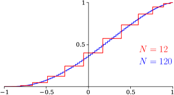
Figure 18.40.1: Histogram approximations to the Repulsive Coulomb–Pollaczek, RCP, weight function integrated over $[-1,x)$, see Figure 18.39.2 for an exact result, for $Z=+1$, shown for $N=12$ and $N=120$. Magnify

… ►Results similar to these appear in Langhoff et al. (1976) in methods developed for physics applications, and which includes treatments of systems with discontinuities in $\mu (x)$, using what is referred to as the Stieltjes derivative which may be traced back to Stieltjes, as discussed by Deltour (1968, Eq. 12). … ►Further, exponential convergence in $N$, via the Derivative Rule, rather than the power-law convergence of the histogram methods, is found for the inversion of Gegenbauer, Attractive, as well as Repulsive, Coulomb–Pollaczek, and Hermite weights and zeros to approximate $w(x)$ for these OP systems on $x\in [-1,1]$ and $(-\mathrm{\infty },\mathrm{\infty })$ respectively, Reinhardt (2018), and Reinhardt (2021b), Reinhardt (2021a). …

24: 18.34 Bessel Polynomials

… ►Hence the full system of polynomials $y_n(x;a)$ cannot be orthogonal on the line with respect to a positive weight function, but this is possible for a finite system of such polynomials, the Romanovski–Bessel polynomials, if : …The full system satisfies orthogonality with respect to a (not positive definite) moment functional; see Evans et al. (1993, (2.7)) for the simple expression of the moments ${\mu }_n$. … ►Orthogonality of the full system on the unit circle can be given with a much simpler weight function: …the integration path being taken in the positive rotational sense. … ►In this limit the finite system of Jacobi polynomials $P_n^{(\alpha ,\beta )}\left(x\right)$ which is orthogonal on $(1,\mathrm{\infty })$ (see §18.3) tends to the finite system of Romanovski–Bessel polynomials which is orthogonal on $(0,\mathrm{\infty })$ (see (18.34.5_5)). …

25: 18.2 General Orthogonal Polynomials

… ►Here $w(x)$ is continuous or piecewise continuous or integrable such that … ►whereas in the latter case the system $\{p_n(x)\}$ is finite: $n=0,1,\mathrm{\dots },N$. … ►Between the systems $\{p_n(x)\}$ and $\{q_n(x)\}$ there are the contiguous relations … ►A system of OP’s with unique orthogonality measure is always complete, see Shohat and Tamarkin (1970, Theorem 2.14). In particular, a system of OP’s on a bounded interval is always complete. …

26: Bibliography R

… ►

ⓘ

Notes:

Symbolic and extended-precision general purpose computer algebra system.

External Links:

Home Page

Referenced by:

§ ‣ Software Cross Index.

Encodings:

BibTeX

… ►

Computation of Hankel (Bessel) functions of complex index and argument by numerical integration of a Schläfli contour integral. Ž. Vyčisl. Mat. i Mat. Fiz. 13, pp. 1415–1424, 1636.

ⓘ

Notes:

English translation in U.S.S.R. Computational Math. and Math. Phys. 13(6), pp. 58–67

External Links:

ISSN 0044-4669, Document, MathReview (H. Zegeling), ZentralBlatt

Referenced by:

§10.74(iii).

Encodings:

BibTeX

… ►

Diffraction of plane radio waves by a parabolic cylinder. Calculation of shadows behind hills. Bell System Tech. J. 33, pp. 417–504.

ⓘ

External Links:

MathReview (J. Shmoys)

Referenced by:

§12.17.

Encodings:

BibTeX

… ►

Elliptic hypergeometric series on root systems. Adv. Math. 181 (2), pp. 417–447.

ⓘ

External Links:

ISSN 0001-8708, Document, MathReview, ZentralBlatt

Referenced by:

§20.11(iii).

Encodings:

BibTeX

…

27: Bibliography K

… ►

The Askey-scheme of hypergeometric orthogonal polynomials and its $q$-analogue. Technical report Technical Report 98-17, Delft University of Technology, Faculty of Information Technology and Systems, Department of Technical Mathematics and Informatics.

ⓘ

External Links:

FullText

Referenced by:

R. Koekoek, P. A. Lesky, and R. F. Swarttouw (2010).

Encodings:

BibTeX

… ►

Comment on “The incomplete beta function law for parallel tempering sampling of classical canonical systems” [J. Chem. Phys. 120, 4119 (2004)]. J. Chem. Phys. 121 (2), pp. 1167.

ⓘ

External Links:

Document

Referenced by:

§8.24(ii).

Encodings:

BibTeX

… ►

Askey-Wilson Polynomials for Root Systems of Type $BC$ . In Hypergeometric Functions on Domains of Positivity, Jack Polynomials, and Applications (Tampa, FL, 1991), Contemp. Math., Vol. 138, pp. 189–204.

ⓘ

External Links:

FullText, MathReview (Eric M. Opdam), ZentralBlatt

Referenced by:

§18.37(iii).

Encodings:

BibTeX

… ►

Algorithm 910: a portable C++ multiple-precision system for special-function calculations. ACM Trans. Math. Software 37 (4), pp. Art. 45, 27.

ⓘ

Notes:

This system provides a uniform interface in C++, named e_float, to perform arithmetic operations and to calculate mathematical functions that are implemented in several different MP packages. It is a free, open-source, multiple precision package that allows the computation of many special functions. It supports calculations with 30….300 decimal digits and is interoperable with Microsoft’s CLR, Python and Mathematica.

External Links:

ISSN 0098-3500, Document, FullText, MathReview Entry, ZentralBlatt

Referenced by:

Erratum (V1.0.9) for References, § ‣ Software Cross Index, § ‣ Software Cross Index, § ‣ Software Cross Index, § ‣ Software Cross Index, § ‣ Software Cross Index, § ‣ Software Cross Index, § ‣ Software Cross Index, § ‣ Software Cross Index, § ‣ Software Cross Index, § ‣ Software Cross Index, § ‣ Software Cross Index, § ‣ Software Cross Index, § ‣ Software Cross Index, § ‣ Software Cross Index, § ‣ Software Cross Index, § ‣ Software Cross Index, § ‣ Software Cross Index, § ‣ Software Cross Index, § ‣ Software Cross Index, § ‣ Software Cross Index, § ‣ Software Cross Index, § ‣ Software Cross Index, § ‣ Software Cross Index, § ‣ Software Cross Index, § ‣ Software Cross Index, § ‣ Software Cross Index, § ‣ Software Cross Index, § ‣ Software Cross Index, § ‣ Software Cross Index, § ‣ Software Cross Index, § ‣ Software Cross Index, § ‣ Software Cross Index.

Encodings:

BibTeX

… ►

The Painlevé-Kowalevski and poly-Painlevé tests for integrability. Stud. Appl. Math. 86 (2), pp. 87–165.

ⓘ

External Links:

ISSN 0022-2526, MathReview (Walter Strampp), ZentralBlatt

Referenced by:

§32.2(i).

Encodings:

BibTeX

…

28: Bibliography M

… ►

Affine root systems and Dedekind’s $\eta$-function. Invent. Math. 15 (2), pp. 91–143.

ⓘ

External Links:

Document, MathReview (D.-N. Verma), ZentralBlatt

Referenced by:

§20.12(i).

Encodings:

BibTeX

►

Some conjectures for root systems. SIAM J. Math. Anal. 13 (6), pp. 988–1007.

ⓘ

External Links:

ISSN 0036-1410, Document, MathReview (S. Milne), ZentralBlatt

Referenced by:

§17.13, §17.14.

Encodings:

BibTeX

… ►

Orthogonal polynomials associated with root systems. Sém. Lothar. Combin. 45, pp. Art. B45a, 40 pp. (electronic).

ⓘ

External Links:

ISSN 1286-4889, FullText, MathReview, ZentralBlatt

Referenced by:

§18.37(iii).

Encodings:

BibTeX

… ►

ⓘ

Notes:

System for the manipulation of symbolic and numerical expressions. Includes a collection of special functions. Utilizes exact fractions, arbitrary precision integers, and arbitrary precision floating point numbers.

External Links:

Home Page

Referenced by:

§ ‣ Software Cross Index, § ‣ Software Cross Index, § ‣ Software Cross Index, § ‣ Software Cross Index, § ‣ Software Cross Index, § ‣ Software Cross Index, § ‣ Software Cross Index, § ‣ Software Cross Index, § ‣ Software Cross Index, § ‣ Software Cross Index, § ‣ Software Cross Index, § ‣ Software Cross Index, § ‣ Software Cross Index, § ‣ Software Cross Index, § ‣ Software Cross Index.

Encodings:

BibTeX

… ►

SciFace Software, Paderborn, Germany.

ⓘ

Notes:

Computer algebra system for doing symbolic and exact algebraic computations as well as numerical calculations with almost arbitrary accuracy

Referenced by:

§ ‣ Software Cross Index.

Encodings:

BibTeX

…

29: 3.7 Ordinary Differential Equations

… ►Assume that we wish to integrate (3.7.1) along a finite path $𝒫$ from $z=a$ to $z=b$ in a domain $D$. … ►If, for example, ${\beta }_0={\beta }_1=0$, then on moving the contributions of $w(z_0)$ and $w(z_P)$ to the right-hand side of (3.7.13) the resulting system of equations is not tridiagonal, but can readily be made tridiagonal by annihilating the elements of ${𝐀}_P$ that lie below the main diagonal and its two adjacent diagonals. … ►The Sturm–Liouville eigenvalue problem is the construction of a nontrivial solution of the system … ►The larger the absolute values of the eigenvalues ${\lambda }_k$ that are being sought, the smaller the integration steps $\left|{\tau }_j\right|$ need to be. …

30: 18.3 Definitions

… ►

With the property that ${\{p_{n+1}^{\prime }(x)\}}_{n=0}^{\mathrm{\infty }}$ is again a system of OP’s. See §18.9(iii).

… ►

Table 18.3.1: Orthogonality properties for classical OP’s: intervals, weight functions, standardizations, leading coefficients, and parameter constraints. …

► ►►

Name	$p_n(x)$	$(a,b)$	$w(x)$	$h_n$	$k_n$	${\tilde{k}}_n/k_n$	Constraints
…

►

… ►For $-1-\beta >\alpha >-1$ a finite system of Jacobi polynomials $P_n^{(\alpha ,\beta )}\left(x\right)$ is orthogonal on $(1,\mathrm{\infty })$ with weight function $w(x)={(x-1)}^{\alpha }{(x+1)}^{\beta }$. For $\nu \in ℝ$ and $N>-\frac{1}{2}$ a finite system of Jacobi polynomials $P_n^{(-N-1+\mathrm{i}\nu ,-N-1-\mathrm{i}\nu )}\left(\mathrm{i}x\right)$ (called pseudo Jacobi polynomials or Routh–Romanovski polynomials) is orthogonal on $(-\mathrm{\infty },\mathrm{\infty })$ with $w(x)={\left(1+x^2\right)}^{-N-1}{\mathrm{e}}^{2\nu \arctan x}$. … ►However, in general they are not orthogonal with respect to a positive measure, but a finite system has such an orthogonality. …