infinite product

SearchAdvancedHelp

(0.001 seconds)

41—49 of 49 matching pages

41: 5.20 Physical Applications

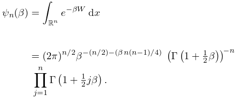
… ►Suppose the potential energy of a gas of $n$ point charges with positions $x_1,x_2,\mathrm{\dots },x_n$ and free to move on the infinite line , is given by … ►

5.20.3 $${\psi }_n(\beta )={\int }_{{ℝ}^n}{\mathrm{e}}^{-\beta W}dx={(2\pi )}^{n/2}{\beta }^{-(n/2)-(\beta n(n-1)/4)}{\left(\mathrm{\Gamma }\left(1+\frac{1}{2}\beta \right)\right)}^{-n}\prod _{j=1}^n\mathrm{\Gamma }\left(1+\frac{1}{2}j\beta \right).$$

ⓘ

Symbols:

$\mathrm{\Gamma }\left(z\right)$: gamma function, $\pi$: the ratio of the circumference of a circle to its diameter, $dx$: differential of $x$ , $\mathrm{e}$: base of natural logarithm, $\int$: integral, $ℝ$: real line, $j$: nonnegative integer, $n$: nonnegative integer, $x$: real variable, $W$: potential energy, ${\psi }_n(\beta )$: partition function and $\beta =1/(kT)$

Permalink:

http://dlmf.nist.gov/5.20.E3

Encodings:

pMML, png, TeX

See also:

Annotations for §5.20, §5.20 and Ch.5

…

42: 27.12 Asymptotic Formulas: Primes

… ►where the series terminates when the product of the first $r$ primes exceeds $x$. … ► $\pi \left(x\right)-\mathrm{li}\left(x\right)$ changes sign infinitely often as $x\to \mathrm{\infty }$; see Littlewood (1914), Bays and Hudson (2000). … ►If $a$ is relatively prime to the modulus $m$, then there are infinitely many primes congruent to $a(modm)$. … ►There are infinitely many Carmichael numbers. …

43: Bibliography W

… ►

Infinitely differentiable generalized logarithmic and exponential functions. Math. Comp. 57 (196), pp. 723–733.

ⓘ

External Links:

ISSN 0025-5718, FullText, Document, MathReview (F. W. J. Olver), ZentralBlatt

Referenced by:

§4.12.

Encodings:

BibTeX

… ►

Reduction formulae for products of theta functions. J. Res. Nat. Inst. Standards and Technology 117, pp. 297–303.

ⓘ

External Links:

Document

Referenced by:

(20.7.34), §20.7(ix).

Encodings:

BibTeX

… ►

The generalised product moment distribution in samples from a normal multivariate population. Biometrika 20A, pp. 32–52.

ⓘ

External Links:

FullText, Document, ZentralBlatt

Referenced by:

§35.3(i), §35.3(ii).

Encodings:

BibTeX

…

44: 28.7 Analytic Continuation of Eigenvalues

… ►The number of branch points is infinite, but countable, and there are no finite limit points. … ►Therefore $w_{\text{I}}^{\prime }(\frac{1}{2}\pi ;a,q)$ is irreducible, in the sense that it cannot be decomposed into a product of entire functions that contain its zeros; see Meixner et al. (1980, p. 88). …

45: 18.36 Miscellaneous Polynomials

… ►Sobolev OP’s are orthogonal with respect to an inner product involving derivatives. … ►This infinite set of polynomials of order $n\ge k$, the smallest power of $x$ being $x^k$ in each polynomial, is a complete orthogonal set with respect to this measure. …

46: Errata

… ►

Factors inside square roots on the right-hand sides of formulas (19.18.6), (19.20.10), (19.20.19), (19.21.7), (19.21.8), (19.21.10), (19.25.7), (19.25.10) and (19.25.11) were written as products to ensure the correct multivalued behavior.

Reported by Luc Maisonobe on 2021-06-07

… ►

The multi-product notation ${(q,c;q)}_m{(q,c^{\prime };q)}_n$ in the denominator of the right-hand side was used.

… ►

20.4.2 $${\theta }_1^{\prime }(0,q)=2q^{1/4}\prod _{n=1}^{\mathrm{\infty }}{\left(1-q^{2n}\right)}^3=2q^{1/4}{(q^2;q^2)}_{\mathrm{\infty }}^3$$

The representation in terms of ${(q^2;q^2)}_{\mathrm{\infty }}^3$ was added to this equation.

… ►

It is now mentioned that (25.2.5), defines the Stieltjes constants ${\gamma }_n$. Consequently, ${\gamma }_n$ in (25.2.4), (25.6.12) are now identified as the Stieltjes constants.

… ►

Some references were added to §§7.25(ii), 7.25(iii), 7.25(vi), 8.28(ii), and to ¶Products (in §10.74(vii)) and §10.77(ix).

…

47: 18.28 Askey–Wilson Class

… ►

18.28.1 $$p_n(x)=p_n(x;a,b,c,d|q)=a^{-n}\sum _{\mathrm{\ell }=0}^n{q}^{\mathrm{\ell }}{(ab{q}^{\mathrm{\ell }},ac{q}^{\mathrm{\ell }},ad{q}^{\mathrm{\ell }};q)}_{n-\mathrm{\ell }}\frac{{(q^{-n},abcd{q}^{n-1};q)}_{\mathrm{\ell }}}{{(q;q)}_{\mathrm{\ell }}}\prod _{j=0}^{\mathrm{\ell }-1}(1-2a{q}^{j}x+a^2{q}^{2j}),$$

ⓘ

Defines:

$p_n(x;a,b,c,d|q)$: Askey–Wilson polynomial

Symbols:

${(a;q)}_n$: $q$-Pochhammer symbol (or $q$-shifted factorial), ${(a_1,a_2,\mathrm{\dots },a_r;q)}_n$: multiple $q$-Pochhammer symbol, $p_n(x)$: polynomial of degree $n$ , $q$: real variable, $\mathrm{\ell }$: nonnegative integer, $n$: nonnegative integer and $x$: real variable

Referenced by:

(18.28.29), §18.28(ii), §18.38(iii), Erratum (V1.2.0) for Equation (18.28.1)

Permalink:

http://dlmf.nist.gov/18.28.E1

Encodings:

pMML, png, TeX

See also:

Annotations for §18.28(ii), §18.28 and Ch.18

… ►

18.28.7 $$Q_n(\cos \theta ;a,b|q)=p_n(\cos \theta ;a,b,0,0|q)=a^{-n}\sum _{\mathrm{\ell }=0}^n{q}^{\mathrm{\ell }}\frac{{(ab{q}^{\mathrm{\ell }};q)}_{n-\mathrm{\ell }}{(q^{-n};q)}_{\mathrm{\ell }}}{{(q;q)}_{\mathrm{\ell }}}\prod _{j=0}^{\mathrm{\ell }-1}(1-2a{q}^j\cos \theta +a^2{q}^{2j})=\frac{{(ab;q)}_n}{a^n}{}_3{}^{}\varphi _2^{}(\genfrac{}{}{0pt}{}{q^{-n},a{\mathrm{e}}^{\mathrm{i}\theta },a{\mathrm{e}}^{-\mathrm{i}\theta }}{ab,0};q,q)={(b{\mathrm{e}}^{-\mathrm{i}\theta };q)}_n{\mathrm{e}}^{\mathrm{i}n\theta }{}_2{}^{}\varphi _1^{}(\genfrac{}{}{0pt}{}{q^{-n},a{\mathrm{e}}^{\mathrm{i}\theta }}{b^{-1}{q}^{1-n}{\mathrm{e}}^{\mathrm{i}\theta }};q,b^{-1}q{\mathrm{e}}^{-\mathrm{i}\theta }).$$

ⓘ

Defines:

$Q_n(x;a,b|q)$: Al-Salam–Chihara polynomial

Symbols:

$p_n(x;a,b,c,d|q)$: Askey–Wilson polynomial, $\cos z$: cosine function, $\mathrm{e}$: base of natural logarithm, $\mathrm{i}$: imaginary unit, ${(a;q)}_n$: $q$-Pochhammer symbol (or $q$-shifted factorial), ${}_{r+1}{}^{}\varphi _s^{}(a_0,\mathrm{\dots },a_r;b_1,\mathrm{\dots },b_s;q,z)$ or ${}_{r+1}{}^{}\varphi _s^{}(\genfrac{}{}{0pt}{}{a_0,\mathrm{\dots },a_r}{b_1,\mathrm{\dots },b_s};q,z)$: basic hypergeometric (or $q$-hypergeometric) function, $q$: real variable, $\mathrm{\ell }$: nonnegative integer, $n$: nonnegative integer and $x$: real variable

Permalink:

http://dlmf.nist.gov/18.28.E7

Encodings:

pMML, png, TeX

See also:

Annotations for §18.28(iii), §18.28 and Ch.18

… ►

18.28.19 $$R_n(x)=R_n(x;\alpha ,\beta ,\gamma ,\delta |q)=\sum _{\mathrm{\ell }=0}^n\frac{q^{\mathrm{\ell }}{(q^{-n},\alpha \beta q^{n+1};q)}_{\mathrm{\ell }}}{{(\alpha q,\beta \delta q,\gamma q,q;q)}_{\mathrm{\ell }}}\prod _{j=0}^{\mathrm{\ell }-1}(1-q^{j}x+\gamma \delta q^{2j+1})={}_4{}^{}\varphi _3^{}(\genfrac{}{}{0pt}{}{q^{-n},\alpha \beta q^{n+1},q^{-y},\gamma \delta q^{y+1}}{\alpha q,\beta \delta q,\gamma q};q,q),$$ $\alpha q$, $\beta \delta q$, or $\gamma q=q^{-N}$; $n=0,1,\mathrm{\dots },N$.

ⓘ

Defines:

$R_n(x;\alpha ,\beta ,\gamma ,\delta |q)$: $q$-Racah polynomial and $R_n(x)$ (locally)

Symbols:

${}_{r+1}{}^{}\varphi _s^{}(a_0,\mathrm{\dots },a_r;b_1,\mathrm{\dots },b_s;q,z)$ or ${}_{r+1}{}^{}\varphi _s^{}(\genfrac{}{}{0pt}{}{a_0,\mathrm{\dots },a_r}{b_1,\mathrm{\dots },b_s};q,z)$: basic hypergeometric (or $q$-hypergeometric) function, ${(a_1,a_2,\mathrm{\dots },a_r;q)}_n$: multiple $q$-Pochhammer symbol, $y$: real variable, $N$: positive integer, $\delta$: arbitrary small positive constant, $q$: real variable, $\mathrm{\ell }$: nonnegative integer, $n$: nonnegative integer and $x$: real variable

Permalink:

http://dlmf.nist.gov/18.28.E19

Encodings:

pMML, png, TeX

See also:

Annotations for §18.28(viii), §18.28 and Ch.18

… ►Leonard (1982) classified all (finite or infinite) discrete systems of OP’s $p_n(x)$ on a set $\{x(m)\}$ for which there is a system of discrete OP’s $q_m(y)$ on a set $\{y(n)\}$ such that $p_n(x(m))=q_m(y(n))$. … ►

18.28.26 $$\underset{\lambda \to 0}{lim}{r}_n(x/(2\lambda );\lambda ,qa{\lambda }^{-1},qc{\lambda }^{-1},b{c}^{-1}\lambda |q)=P_n(x;a,b,c;q).$$

ⓘ

Symbols:

$P_n(x;a,b,c;q)$: big $q$-Jacobi polynomial, ${(a_1,a_2,\mathrm{\dots },a_r;q)}_n$: multiple $q$-Pochhammer symbol, $z$: complex variable, $q$: real variable, $\mathrm{\ell }$: nonnegative integer, $n$: nonnegative integer and $x$: real variable

Source:

Koekoek et al. (2010, (14.1.18))

Proof sketch:

In the terminating $q$-hypergeometric series which defines the ${}_4{}^{}\varphi _3^{}$ in (18.28.1_5), with ${(az{q}^{\mathrm{\ell }},a{z}^{-1}{q}^{\mathrm{\ell }};q)}_{\mathrm{\ell }}$ written as ${\prod }_{j=0}^{\mathrm{\ell }-1}(1-2a{q}^{j}x+a^2{q}^{2j})$, substitute for $x$ and the parameters according to the left-hand side of the present formula, take the limit, and obtain the ${}_3{}^{}\varphi _2^{}$ as in (18.27.5).

Referenced by:

(18.28.27), (18.28.28), §18.28(x)

Permalink:

http://dlmf.nist.gov/18.28.E26

Encodings:

pMML, png, TeX

See also:

Annotations for §18.28(x), §18.28(x), §18.28 and Ch.18

…

48: 18.39 Applications in the Physical Sciences

… ►with an infinite set of orthonormal $L^2$ eigenfunctions … ►This indicates that the Laguerre polynomials appearing in (18.39.29) are not classical OP’s, and in fact, even though infinite in number for fixed $l$, do not form a complete set. Namely for fixed $l$ the infinite set labeled by $p$ describe only the $L^2$ bound states for that single $l$, omitting the continuum briefly mentioned below, and which is the subject of Chapter 33, and so an unusual example of the mixed spectra of §1.18(viii). … ►These, taken together with the infinite sets of bound states for each $l$, form complete sets. … ►The fact that non-$L^2$ continuum scattering eigenstates may be expressed in terms or (infinite) sums of $L^2$ functions allows a reformulation of scattering theory in atomic physics wherein no non-$L^2$ functions need appear. …

49: 3.5 Quadrature

… ►The nodes $x_1,x_2,\mathrm{\dots },x_n$ are prescribed, and the weights $w_k$ and error term $E_n(f)$ are found by integrating the product of the Lagrange interpolation polynomial of degree $n-1$ and $w(x)$. … ►Let $\{p_n\}$ denote the set of monic polynomials $p_n$ of degree $n$ (coefficient of $x^n$ equal to $1$) that are orthogonal with respect to a positive weight function $w$ on a finite or infinite interval $(a,b)$; compare §18.2(i). … ►For computing infinite oscillatory integrals, Longman’s method may be used. …