improved

SearchAdvancedHelp

(0.000 seconds)

31—40 of 57 matching pages

31: 5.17 Barnes’ $G$-Function (Double Gamma Function)

… ►For error bounds and an exponentially-improved extension, see Nemes (2014a). …

32: Bibliography V

… ►

Improved calculation of prolate spheroidal radial functions of the second kind and their first derivatives. Quart. Appl. Math. 62 (3), pp. 493–507.

ⓘ

Notes:

For software, see Van Buren (website)

External Links:

ISSN 0033-569X, FullText, MathReview (Javier Segura), ZentralBlatt

Referenced by:

§30.16(iii), §30.16(iii).

Encodings:

BibTeX

…

33: 11.11 Asymptotic Expansions of Anger–Weber Functions

… ►For sharp error bounds and exponentially-improved extensions, see Nemes (2018). … ►The later references also contain exponentially-improved extensions of (11.11.8) and (11.11.10). …

34: 9.7 Asymptotic Expansions

… ►

§9.7(v) Exponentially-Improved Expansions

…

35: 10.74 Methods of Computation

… ►Furthermore, the attainable accuracy can be increased substantially by use of the exponentially-improved expansions given in §10.17(v), even more so by application of the hyperasymptotic expansions to be found in the references in that subsection. …

36: 13.29 Methods of Computation

… ►However, this accuracy can be increased considerably by use of the exponentially-improved forms of expansion supplied by the combination of (13.7.10) and (13.7.11), or by use of the hyperasymptotic expansions given in Olde Daalhuis and Olver (1995a). …

37: 19.14 Reduction of General Elliptic Integrals

… ►It then improves the classical method by first applying Hermite reduction to (19.2.3) to arrive at integrands without multiple poles and uses implicit full partial-fraction decomposition and implicit root finding to minimize computing with algebraic extensions. …

38: 25.14 Lerch’s Transcendent

… ►

25.14.6 $$\mathrm{\Phi }(z,s,a)=\frac{1}{2}{a}^{-s}+{\int }_0^{\mathrm{\infty }}\frac{z^x}{{(a+x)}^s}dx-2{\int }_0^{\mathrm{\infty }}\frac{\sin \left(x\ln z-s\arctan \left(x/a\right)\right)}{{(a^2+x^2)}^{s/2}({\mathrm{e}}^{2\pi x}-1)}dx,$$ $\mathrm{\Re }a>0$ if ; $\mathrm{\Re }s>1$, $\mathrm{\Re }a>0$ if $\left|z\right|=1$.

ⓘ

Symbols:

$\mathrm{\Phi }(z,s,a)$: Lerch’s transcendent, $\pi$: the ratio of the circumference of a circle to its diameter, $dx$: differential of $x$ , $\mathrm{e}$: base of natural logarithm, $\int$: integral, $\arctan z$: arctangent function, $\ln z$: principal branch of logarithm function, $\mathrm{\Re }$: real part, $\sin z$: sine function, $x$: real variable, $a$: real or complex parameter, $s$: complex variable and $z$: complex variable

Keywords:

improper integral, integral representation

Source:

Erdélyi et al. (1953a, (1.11.4), p. 28)

Notes:

For the case see Erdélyi et al. (1953a, (1.11.4), p. 28). In the case $\left|z\right|=1$ one checks that the first integral converges absolutely iff $\mathrm{\Re }s>1$.

Referenced by:

Erratum (V1.1.4) for Equation (25.14.6)

Permalink:

http://dlmf.nist.gov/25.14.E6

Encodings:

pMML, png, TeX

Clarification (effective with 1.1.4):

The constraint which originally read “$\mathrm{\Re }s>0$ if ; $\mathrm{\Re }s>1$ if $|z|=1,\mathrm{\Re }a>0$” has been improved to be “$\mathrm{\Re }a>0$ if ; $\mathrm{\Re }s>1$, $\mathrm{\Re }a>0$ if $\left|z\right|=1$”.

Suggested 2021-08-23 by Gergő Nemes

See also:

Annotations for §25.14(ii), §25.14 and Ch.25

…

39: 30.16 Methods of Computation

… ►Approximations to eigenvalues can be improved by using the continued-fraction equations from §30.3(iii) and §30.8; see Bouwkamp (1947) and Meixner and Schäfke (1954, §3.93). …

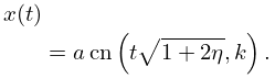
40: 22.19 Physical Applications

… ►

22.19.6 $$x(t)=a\mathrm{cn}(t\sqrt{1+2\eta },k).$$

ⓘ

Symbols:

$\mathrm{cn}(z,k)$: Jacobian elliptic function, $k$: modulus, $x(t)$: coordinate, $t$: time, $a$: displacement and $\eta$: parameter

Referenced by:

Erratum (V1.0.9) for Equation (22.19.6), Erratum (V1.0.9) for Equations (22.19.6), (22.19.7), (22.19.8), (22.19.9)

Permalink:

http://dlmf.nist.gov/22.19.E6

Encodings:

pMML, png, TeX

Errata (effective with 1.0.9):

Originally the term $\sqrt{1+2\eta }$ was given incorrectly as $\sqrt{1+\eta }$ in this equation and in the line above. Additionally, for improved clarity, the modulus $k$ has been defined in the line above. Previously $1/\sqrt{2+{\eta }^{-1}}$ was given explicitly in the equation.

Reported 2014-04-28 by Svante Janson

See also:

Annotations for §22.19(ii), §22.19(ii), §22.19 and Ch.22

…