…
►
►‘✓’ indicates that a software package implements the
functions in a section; ‘
a’ indicates available
functionality through optional or add-on packages; an empty space indicates no known support.
…
►In the list below we identify four main sources of software for computing special
functions.
…
►
Commercial Software.
Such software ranges from a collection of reusable software
parts (e.g., a library) to fully functional interactive computing environments
with an associated computing language. Such software is usually professionally
developed, tested, and maintained to high standards. It is available for purchase,
often with accompanying updates and consulting support.
…
►The following are web-based software repositories with significant holdings in the area of special
functions.
…
…
►Usually, however, other methods are more efficient, especially the numerical solution of difference
equations (§
3.6) and the application of uniform asymptotic expansions (when available) for OP’s of large degree.
…
…
►There are many ways to implement these first two steps, noting that the expressions for
and
of
equation (
18.2.30) are of little practical numerical value, see
Gautschi (2004) and
Golub and Meurant (2010).
…
►Results of low (
to
decimal digits) precision for
are easily obtained for
to
.
…
►Equation (
18.40.7) provides step-histogram approximations to
, as shown in Figure
18.40.1 for
and
, shown here for the repulsive Coulomb–Pollaczek OP’s of Figure
18.39.2, with the parameters as listed therein.
…
§7.8 Inequalities
…
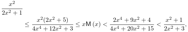
►
7.8.5
.
…
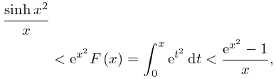
►
7.8.7
.
►The
function
is strictly decreasing for
.
…
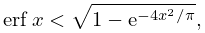
►
7.8.8
.
§20.11 Generalizations and Analogs
…
►The first of
equations (
20.9.2) can also be written
…
►
§20.11(iv) Theta Functions with Characteristics
…
►The importance of these combined theta
functions is that sets of twelve
equations for the theta
functions often can be replaced by corresponding sets of three
equations of the combined theta
functions, plus permutation symmetry.
Such sets of twelve
equations include derivatives, differential
equations, bisection relations, duplication relations, addition formulas (including new ones for theta
functions), and pseudo-addition formulas.
…
…
►
also controls time evolution of the
wave function
via the
time-dependent Schrödinger
equation,
…
►Substitution of (
18.39.24) into (
18.39.23) then gives the ordinary differential
equation for the
radial wave function
,
…
►The non-relativistic Schrödinger
equation describing a single, bound (negative energy) electron, in an
eigenstate of energy
is:
…
►The
functions
satisfy the
equation,
…
►
Discretized and Continuum Expansions of Scattering Eigenfunctions in terms of Pollaczek Polynomials: J-matrix Theory
…
