formally self adjoint linear operator

SearchAdvancedHelp

(0.001 seconds)

11—20 of 155 matching pages

11: 3.10 Continued Fractions

… ►Every convergent, asymptotic, or formal series … ►We say that it corresponds to the formal power series … ►We say that it is associated with the formal power series $f(z)$ in (3.10.7) if the expansion of its $n$th convergent $C_n$ in ascending powers of $z$, agrees with (3.10.7) up to and including the term in $z^{2n-1}$, $n=1,2,3,\mathrm{\dots }$. … ►($\nabla$ is the backward difference operator.) …

12: 16.11 Asymptotic Expansions

… ►

§16.11(i) Formal Series

►For subsequent use we define two formal infinite series, $E_{p,q}(z)$ and $H_{p,q}(z)$, as follows: ►

16.11.1 $$E_{p,q}(z)={(2\pi )}^{(p-q)/2}{\kappa }^{-\nu -(1/2)}{\mathrm{e}}^{\kappa z^{1/\kappa }}\sum _{k=0}^{\mathrm{\infty }}{c}_k{\left(\kappa z^{1/\kappa }\right)}^{\nu -k},$$ ,

ⓘ

Defines:

$E_{p,q}(z)$: formal infinite series (locally)

Symbols:

$\pi$: the ratio of the circumference of a circle to its diameter, $\mathrm{e}$: base of natural logarithm, $p$: nonnegative integer, $q$: nonnegative integer, $z$: complex variable, $\kappa$ and $\nu$

Referenced by:

§16.11(i), §16.11(ii)

Permalink:

http://dlmf.nist.gov/16.11.E1

Encodings:

pMML, png, TeX

See also:

Annotations for §16.11(i), §16.11 and Ch.16

►

16.11.2 $$H_{p,q}(z)=\sum _{m=1}^p\sum _{k=0}^{\mathrm{\infty }}\frac{{(-1)}^k}{k!}\mathrm{\Gamma }\left(a_m+k\right)\left(\prod _{\begin{array}{c}\mathrm{\ell }=1\\ \mathrm{\ell }\ne m\end{array}}^p\mathrm{\Gamma }\left(a_{\mathrm{\ell }}-a_m-k\right)/\prod _{\mathrm{\ell }=1}^q\mathrm{\Gamma }\left(b_{\mathrm{\ell }}-a_m-k\right)\right)z^{-a_m-k}.$$

ⓘ

Defines:

$H_{p,q}(z)$: formal infinite series (locally)

Symbols:

$\mathrm{\Gamma }\left(z\right)$: gamma function, $!$: factorial (as in $n!$), $p$: nonnegative integer, $q$: nonnegative integer, $z$: complex variable, $a,a_1,\mathrm{\dots },a_p$: real or complex parameters and $b,b_1,\mathrm{\dots },b_q$: real or complex parameters

Referenced by:

§16.11(ii), §16.11(ii)

Permalink:

http://dlmf.nist.gov/16.11.E2

Encodings:

pMML, png, TeX

See also:

Annotations for §16.11(i), §16.11 and Ch.16

… ►The formal series (16.11.2) for $H_{q+1,q}(z)$ converges if $\left|z\right|>1$, and …

13: 1.17 Integral and Series Representations of the Dirac Delta

… ►Formal interchange of the order of integration in the Fourier integral formula ((1.14.1) and (1.14.4)): …Then comparison of (1.17.2) and (1.17.9) yields the formal integral representation … ►In the language of physics and applied mathematics, these equations indicate the normalizations chosen for these non-$L^2$ improper eigenfunctions of the differential operators (with derivatives respect to spatial co-ordinates) which generate them; the normalizations (1.17.12_1) and (1.17.12_2) are explicitly derived in Friedman (1990, Ch. 4), the others follow similarly. … ►Formal interchange of the order of summation and integration in the Fourier summation formula ((1.8.3) and (1.8.4)): … ►By analogy with §1.17(ii) we have the formal series representation …

14: How to Cite

… ►When citing DLMF from a formal publication, we suggest a format similar to the following: …

15: Bibliography K

… ►

Quasi-linear Stokes phenomenon for the Painlevé first equation. J. Phys. A 37 (46), pp. 11149–11167.

ⓘ

External Links:

ISSN 0305-4470, Document, MathReview (W. Balser), ZentralBlatt

Referenced by:

§32.12(i).

Encodings:

BibTeX

… ►

Linear convergence and the bisection algorithm. Amer. Math. Monthly 93 (1), pp. 48–51.

ⓘ

External Links:

ISSN 0002-9890, FullText, MathReview (J. G. Herriot), ZentralBlatt

Referenced by:

§3.8(iii).

Encodings:

BibTeX

… ►

Lowering and Raising Operators for Some Special Orthogonal Polynomials. In Jack, Hall-Littlewood and Macdonald Polynomials, Contemp. Math., Vol. 417, pp. 227–238.

ⓘ

External Links:

FullText, MathReview Entry, ZentralBlatt

Referenced by:

§18.9(iii).

Encodings:

BibTeX

… ►

An algorithm for solving second order linear homogeneous differential equations. J. Symbolic Comput. 2 (1), pp. 3–43.

ⓘ

External Links:

ISSN 0747-7171, MathReview, ZentralBlatt

Referenced by:

§31.14(ii).

Encodings:

BibTeX

… ►

Quantum-Theoretical Formalism for Inhomogeneous Graded-Index Waveguides. Akademie Verlag, Berlin-New York.

ⓘ

External Links:

ISBN 3-05-501598-3, MathReview (Apostolos Vourdas), ZentralBlatt

Referenced by:

§10.73(i).

Encodings:

BibTeX

…

16: DLMF Project News

error generating summary

17: 10.70 Zeros

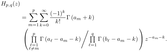
… ►Let $\mu =4{\nu }^2$ and $f(t)$ denote the formal series …

18: Bibliography B

… ►

Transcendental Functions Satisfying Nonhomogeneous Linear Differential Equations. The Macmillan Co., New York.

ⓘ

External Links:

MathReview (H. Hochstadt), ZentralBlatt

Referenced by:

§11.4(i), §11.4(v), §11.5(ii), §11.5(i), §11.5(ii), §11.5(iii), §11.7(ii), §11.7(iii), §11.7(v), §11.9(i), §11.9(iv), §11.9(iv), Ch.11, §14.29.

Encodings:

BibTeX

… ►

An Introduction to Linear Difference Equations. Dover Publications Inc., New York.

ⓘ

Notes:

Unaltered republication of the original 1927 Harvard University edition.

External Links:

MathReview, ZentralBlatt

Referenced by:

§8.1, Notations P, Notations Q.

Encodings:

BibTeX

… ►

Formal Power Series and Algebraic Combinatorics. DIMACS Series in Discrete Mathematics and Theoretical Computer Science, Vol. 24, American Mathematical Society, Providence, RI.

ⓘ

External Links:

ISBN 0-8218-0324-7, MathReview, ZentralBlatt

Referenced by:

§26.19.

Encodings:

BibTeX

… ►

Discrete ordinate solution of Fokker-Planck equations with non-linear coefficients. Phys. Rev. A 31 (3), pp. 1855–1868.

ⓘ

Referenced by:

§18.39(iii).

Encodings:

BibTeX

… ►

Error estimates for the solution of linear systems. SIAM J. Sci. Comput. 21 (2), pp. 764–781.

ⓘ

External Links:

ISSN 1095-7197, Document, MathReview (Dimitrios Noutsos), ZentralBlatt

Referenced by:

§3.2(iii).

Encodings:

BibTeX

…

19: 2.3 Integrals of a Real Variable

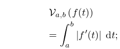
… ►In both cases the $n$th error term is bounded in absolute value by $x^{-n}{𝒱}_{a,b}\left(q^{(n-1)}(t)\right)$, where the variational operator ${𝒱}_{a,b}$ is defined by ►

2.3.6 $${𝒱}_{a,b}\left(f(t)\right)={\int }_a^b\left|f^{\prime }(t)\right|dt;$$

ⓘ

Symbols:

$dx$: differential of $x$ , $\int$: integral, ${𝒱}_{a,b}\left(f\right)$: total variation, $a$: left endpoint and $b$: right endpoint

Referenced by:

§10.17(iv), Erratum (V1.1.1) for Equation (2.3.6)

Permalink:

http://dlmf.nist.gov/2.3.E6

Encodings:

pMML, png, TeX

Correction (effective with 1.1.1):

The integrand was corrected so that the absolute value does not include the differential.

Suggested 2021-02-08 by Juan Luis Varona

See also:

Annotations for §2.3(i), §2.3 and Ch.2

… ►Then the series obtained by substituting (2.3.7) into (2.3.1) and integrating formally term by term yields an asymptotic expansion: … ►The desired uniform expansion is then obtained formally as in Watson’s lemma and Laplace’s method. …

20: 18.2 General Orthogonal Polynomials

… ►

§18.2(ii) $x$-Difference Operators

… ►It is to be noted that, although formally correct, the results of (18.2.30) are of little utility for numerical work, as Hankel determinants are notoriously ill-conditioned. … ►where $f(t)$ and $u(t)$ are formal power series in $t$, with $f(0)=1$, $u(0)=0$ and $u^{\prime }(0)=1$. …If $v(s)$ is the formal power series such that $v(u(t))=t$ then a property equivalent to (18.2.45) with $c_n=1$ is that … …