first

SearchAdvancedHelp

(0.001 seconds)

31—40 of 417 matching pages

31: 14.22 Graphics

… ►

►

►

Figure 14.22.1: $P_{1/2}^0\left(x+\mathrm{i}y\right)$, $-5\le x\le 5$, $-5\le y\le 5$. … Magnify 3D Help

►

►

►

Figure 14.22.2: $P_{1/2}^{-1/2}\left(x+\mathrm{i}y\right)$, $-5\le x\le 5$, $-5\le y\le 5$. … Magnify 3D Help

►

►

►

Figure 14.22.3: $P_{1/2}^{-1}\left(x+\mathrm{i}y\right)$, $-5\le x\le 5$, $-5\le y\le 5$. … Magnify 3D Help

…

32: 29.16 Asymptotic Expansions

… ►The approximations for Lamé polynomials hold uniformly on the rectangle $0\le \mathrm{\Re }z\le K$, $0\le \mathrm{\Im }z\le K^{\prime }$, when $nk$ and $n{k}^{\prime }$ assume large real values. …

33: 22.5 Special Values

… ►Table 22.5.1 gives the value of each of the 12 Jacobian elliptic functions, together with its $z$-derivative (or at a pole, the residue), for values of $z$ that are integer multiples of $K$, $\mathrm{i}{K}^{\prime }$. For example, at $z=K+\mathrm{i}{K}^{\prime }$, $\mathrm{sn}(z,k)=1/k$, $d\mathrm{sn}(z,k)/dz=0$. … ►If $k\to 0+$, then $K\to \pi /2$ and $K^{\prime }\to \mathrm{\infty }$; if $k\to 1-$, then $K\to \mathrm{\infty }$ and $K^{\prime }\to \pi /2$. … ►Expansions for $K,K^{\prime }$ as $k\to 0$ or $1$ are given in §§19.5, 19.12. ►For values of $K,K^{\prime }$ when $k^2=\frac{1}{2}$ (lemniscatic case) see §23.5(iii), and for $k^2={\mathrm{e}}^{\mathrm{i}\pi /3}$ (equianharmonic case) see §23.5(v). …

34: 10.45 Functions of Imaginary Order

… ►and ${\tilde{I}}_{\nu }\left(x\right)$, ${\tilde{K}}_{\nu }\left(x\right)$ are real and linearly independent solutions of (10.45.1): … ►In consequence of (10.45.5)–(10.45.7), ${\tilde{I}}_{\nu }\left(x\right)$ and ${\tilde{K}}_{\nu }\left(x\right)$ comprise a numerically satisfactory pair of solutions of (10.45.1) when $x$ is large, and either ${\tilde{I}}_{\nu }\left(x\right)$ and $(1/\pi )\sinh \left(\pi \nu \right){\tilde{K}}_{\nu }\left(x\right)$, or ${\tilde{I}}_{\nu }\left(x\right)$ and ${\tilde{K}}_{\nu }\left(x\right)$, comprise a numerically satisfactory pair when $x$ is small, depending whether $\nu \ne 0$ or $\nu =0$. … ►For graphs of ${\tilde{I}}_{\nu }\left(x\right)$ and ${\tilde{K}}_{\nu }\left(x\right)$ see §10.26(iii). ►For properties of ${\tilde{I}}_{\nu }\left(x\right)$ and ${\tilde{K}}_{\nu }\left(x\right)$, including uniform asymptotic expansions for large $\nu$ and zeros, see Dunster (1990a). In this reference ${\tilde{I}}_{\nu }\left(x\right)$ is denoted by $(1/\pi )\sinh \left(\pi \nu \right)L_{\mathrm{i}\nu }(x)$. …

35: 10.31 Power Series

… ►For $I_{\nu }\left(z\right)$ see (10.25.2) and (10.27.1). … ►

10.31.1 $$K_n\left(z\right)=\frac{1}{2}{(\frac{1}{2}z)}^{-n}\sum _{k=0}^{n-1}\frac{(n-k-1)!}{k!}{(-\frac{1}{4}{z}^2)}^k+{(-1)}^{n+1}\ln \left(\frac{1}{2}z\right)I_n\left(z\right)+{(-1)}^n\frac{1}{2}{(\frac{1}{2}z)}^n\sum _{k=0}^{\mathrm{\infty }}\left(\psi \left(k+1\right)+\psi \left(n+k+1\right)\right)\frac{{(\frac{1}{4}{z}^2)}^k}{k!(n+k)!},$$

ⓘ

Symbols:

$\psi \left(z\right)$: psi (or digamma) function, $!$: factorial (as in $n!$), $I_{\nu }\left(z\right)$: modified Bessel function of the first kind, $K_{\nu }\left(z\right)$: modified Bessel function of the second kind, $\ln z$: principal branch of logarithm function, $n$: integer, $k$: nonnegative integer and $z$: complex variable

A&S Ref:

9.6.11

Referenced by:

§10.30(i), §10.65(ii)

Permalink:

http://dlmf.nist.gov/10.31.E1

Encodings:

pMML, png, TeX

See also:

Annotations for §10.31 and Ch.10

… ►

10.31.2 $$K_0\left(z\right)=-\left(\ln \left(\frac{1}{2}z\right)+\gamma \right)I_0\left(z\right)+\frac{\frac{1}{4}{z}^2}{{(1!)}^2}+(1+\frac{1}{2})\frac{{(\frac{1}{4}{z}^2)}^2}{{(2!)}^2}+(1+\frac{1}{2}+\frac{1}{3})\frac{{(\frac{1}{4}{z}^2)}^3}{{(3!)}^2}+\mathrm{\cdots }.$$

ⓘ

Symbols:

$\gamma$: Euler’s constant, $!$: factorial (as in $n!$), $I_{\nu }\left(z\right)$: modified Bessel function of the first kind, $K_{\nu }\left(z\right)$: modified Bessel function of the second kind, $\ln z$: principal branch of logarithm function and $z$: complex variable

A&S Ref:

9.6.13

Referenced by:

§10.45

Permalink:

http://dlmf.nist.gov/10.31.E2

Encodings:

pMML, png, TeX

See also:

Annotations for §10.31 and Ch.10

… ►

10.31.3 $$I_{\nu }\left(z\right)I_{\mu }\left(z\right)={(\frac{1}{2}z)}^{\nu +\mu }\sum _{k=0}^{\mathrm{\infty }}\frac{{\left(\nu +\mu +k+1\right)}_k{(\frac{1}{4}{z}^2)}^k}{k!\mathrm{\Gamma }\left(\nu +k+1\right)\mathrm{\Gamma }\left(\mu +k+1\right)}.$$

ⓘ

Symbols:

$\mathrm{\Gamma }\left(z\right)$: gamma function, ${\left(a\right)}_n$: Pochhammer’s symbol (or shifted factorial), $!$: factorial (as in $n!$), $I_{\nu }\left(z\right)$: modified Bessel function of the first kind, $k$: nonnegative integer, $z$: complex variable and $\nu$: complex parameter

Referenced by:

§10.31

Permalink:

http://dlmf.nist.gov/10.31.E3

Encodings:

pMML, png, TeX

Correction (effective with 1.1.2):

The Pochhammer symbol now links to its definition.

See also:

Annotations for §10.31 and Ch.10

36: 22.1 Special Notation

… ► ►►►►

$x,y$	real variables.
…
$K$, $K^{\prime }$	$K\left(k\right)$, $K^{\prime }\left(k\right)=K\left(k^{\prime }\right)$ (complete elliptic integrals of the first kind (§19.2(ii))).
…
$\tau$	$\mathrm{i}{K}^{\prime }/K$.

…

37: 19.7 Connection Formulas

… ►

§19.7(i) Complete Integrals of the First and Second Kinds

… ►

19.7.1 $$E\left(k\right)K^{\prime }\left(k\right)+E^{\prime }\left(k\right)K\left(k\right)-K\left(k\right)K^{\prime }\left(k\right)=\frac{1}{2}\pi .$$

ⓘ

Symbols:

$\pi$: the ratio of the circumference of a circle to its diameter, $K^{\prime }\left(k\right)$: Legendre’s complementary complete elliptic integral of the first kind, $E^{\prime }\left(k\right)$: Legendre’s complementary complete elliptic integral of the second kind, $K\left(k\right)$: Legendre’s complete elliptic integral of the first kind, $E\left(k\right)$: Legendre’s complete elliptic integral of the second kind and $k$: real or complex modulus

Referenced by:

§19.21(i), §19.35(i), §19.7(i)

Permalink:

http://dlmf.nist.gov/19.7.E1

Encodings:

pMML, png, TeX

See also:

Annotations for §19.7(i), §19.7(i), §19.7 and Ch.19

… ►

$$K\left(1/k\right)=k(K\left(k\right)\mp \mathrm{i}K\left(k^{\prime }\right)),$$

►

$$K\left(1/k^{\prime }\right)=k^{\prime }(K\left(k^{\prime }\right)\pm \mathrm{i}K\left(k\right)),$$

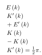
… ►The first of the three relations maps each circular region onto itself and each hyperbolic region onto the other; in particular, it gives the Cauchy principal value of $\mathrm{\Pi }(\varphi ,{\alpha }^2,k)$ when ${\alpha }^2>{\csc }^2\varphi$ (see (19.6.5) for the complete case). …

38: 14.28 Sums

… ►

14.28.1 $$P_{\nu }\left(z_1{z}_2-{\left(z_1^2-1\right)}^{1/2}{\left(z_2^2-1\right)}^{1/2}\cos \varphi \right)=P_{\nu }\left(z_1\right)P_{\nu }\left(z_2\right)+2\sum _{m=1}^{\mathrm{\infty }}{(-1)}^m\frac{\mathrm{\Gamma }\left(\nu -m+1\right)}{\mathrm{\Gamma }\left(\nu +m+1\right)}{P}_{\nu }^m\left(z_1\right)P_{\nu }^m(z_2)\cos \left(m\varphi \right),$$

ⓘ

Symbols:

$\mathrm{\Gamma }\left(z\right)$: gamma function, $P_{\nu }^{\mu }\left(z\right)$: associated Legendre function of the first kind, $\cos z$: cosine function, $P_{\nu }\left(z\right)=P_{\nu }^0\left(z\right)$: Legendre function of the first kind, $z$: complex variable, $m$: nonnegative integer and $\nu$: general degree

Permalink:

http://dlmf.nist.gov/14.28.E1

Encodings:

pMML, png, TeX

See also:

Annotations for §14.28(i), §14.28 and Ch.14

… ►

14.28.2 $$\sum _{n=0}^{\mathrm{\infty }}(2n+1)Q_n\left(z_1\right)P_n\left(z_2\right)=\frac{1}{z_1-z_2},$$ $z_1\in {ℰ}_1$, $z_2\in {ℰ}_2$,

ⓘ

Symbols:

$\in$: element of, $P_{\nu }\left(z\right)=P_{\nu }^0\left(z\right)$: Legendre function of the first kind, $Q_{\nu }\left(z\right)=Q_{\nu }^0\left(z\right)$: Legendre function of the second kind, $z$: complex variable, $n$: nonnegative integer and ${ℰ}_1$, ${ℰ}_2$: ellipses

Permalink:

http://dlmf.nist.gov/14.28.E2

Encodings:

pMML, png, TeX

See also:

Annotations for §14.28(ii), §14.28 and Ch.14

…

39: 19.4 Derivatives and Differential Equations

… ►

${\displaystyle \frac{dK\left(k\right)}{dk}}={\displaystyle \frac{E\left(k\right)-k_{}^{\prime }{}_{}{}^{2}K\left(k\right)}{kk_{}^{\prime }{}_{}{}^2}},$

►

${\displaystyle \frac{d(E\left(k\right)-k_{}^{\prime }{}_{}{}^{2}K\left(k\right))}{dk}}=kK\left(k\right),$

►

${\displaystyle \frac{dE\left(k\right)}{dk}}={\displaystyle \frac{E\left(k\right)-K\left(k\right)}{k}},$

… ►

19.4.3 $$\frac{d^{2}E\left(k\right)}{{dk}^2}=-\frac{1}{k}\frac{dK\left(k\right)}{dk}=\frac{k_{}^{\prime }{}_{}{}^{2}K\left(k\right)-E\left(k\right)}{k^{2}k_{}^{\prime }{}_{}{}^2},$$

ⓘ

Symbols:

$K\left(k\right)$: Legendre’s complete elliptic integral of the first kind, $E\left(k\right)$: Legendre’s complete elliptic integral of the second kind, $\frac{df}{dx}$: derivative of $f$ with respect to $x$ , $k$: real or complex modulus and $k^{\prime }$: complementary modulus

Permalink:

http://dlmf.nist.gov/19.4.E3

Encodings:

pMML, png, TeX

See also:

Annotations for §19.4(i), §19.4 and Ch.19

… ►If $\varphi =\pi /2$, then these two equations become hypergeometric differential equations (15.10.1) for $K\left(k\right)$ and $E\left(k\right)$. …

40: 10.66 Expansions in Series of Bessel Functions

… ►

10.66.1 $${\mathrm{ber}}_{\nu }x+\mathrm{i}{\mathrm{bei}}_{\nu }x=\sum _{k=0}^{\mathrm{\infty }}\frac{{\mathrm{e}}^{(3\nu +k)\pi \mathrm{i}/4}{x}^k{J}_{\nu +k}\left(x\right)}{2^{k/2}k!}=\sum _{k=0}^{\mathrm{\infty }}\frac{{\mathrm{e}}^{(3\nu +3k)\pi \mathrm{i}/4}{x}^k{I}_{\nu +k}\left(x\right)}{2^{k/2}k!}.$$

ⓘ

Symbols:

$J_{\nu }\left(z\right)$: Bessel function of the first kind, ${\mathrm{bei}}_{\nu }\left(x\right)$: Kelvin function, ${\mathrm{ber}}_{\nu }\left(x\right)$: Kelvin function, $\pi$: the ratio of the circumference of a circle to its diameter, $\mathrm{e}$: base of natural logarithm, $!$: factorial (as in $n!$), $\mathrm{i}$: imaginary unit, $I_{\nu }\left(z\right)$: modified Bessel function of the first kind, $k$: nonnegative integer, $x$: real variable and $\nu$: complex parameter

A&S Ref:

9.9.32

Referenced by:

§10.66

Permalink:

http://dlmf.nist.gov/10.66.E1

Encodings:

pMML, png, TeX

See also:

Annotations for §10.66 and Ch.10

►

${\mathrm{ber}}_n\left(x\sqrt{2}\right)={\displaystyle \sum _{k=-\mathrm{\infty }}^{\mathrm{\infty }}}{(-1)}^{n+k}{J}_{n+2k}\left(x\right)I_{2k}\left(x\right),$

►

${\mathrm{bei}}_n\left(x\sqrt{2}\right)={\displaystyle \sum _{k=-\mathrm{\infty }}^{\mathrm{\infty }}}{(-1)}^{n+k}{J}_{n+2k+1}\left(x\right)I_{2k+1}\left(x\right).$