finite sum of 3j symbols

SearchAdvancedHelp

(0.009 seconds)

1—10 of 23 matching pages

1: 34.6 Definition: $\mathit{9}j$ Symbol

… ►The $\mathit{9}j$ symbol may be defined either in terms of $\mathit{3}j$ symbols or equivalently in terms of $\mathit{6}j$ symbols: ►

34.6.1

ⓘ

Defines:

: $\mathit{9}j$ symbol

Symbols:

: $\mathit{3}j$ symbol, $j,j_r$: non-negative integers or non-negative integers plus one half., $r$: nonnegative integer and $s$: integer

Permalink:

http://dlmf.nist.gov/34.6.E1

Encodings:

pMML, png, TeX

See also:

Annotations for §34.6 and Ch.34

…

2: 34.4 Definition: $\mathit{6}j$ Symbol

§34.4 Definition: $\mathit{6}j$ Symbol

… ►For alternative expressions for the $\mathit{6}j$ symbol, written either as a finite sum or as other terminating generalized hypergeometric series ${}_4{}^{}F_3^{}$ of unit argument, see Varshalovich et al. (1988, §§9.2.1, 9.2.3).

3: 34.2 Definition: $\mathit{3}j$ Symbol

… ►When both conditions are satisfied the $\mathit{3}j$ symbol can be expressed as the finite sum … ►where ${}_3{}^{}F_2^{}$ is defined as in §16.2. ►For alternative expressions for the $\mathit{3}j$ symbol, written either as a finite sum or as other terminating generalized hypergeometric series ${}_3{}^{}F_2^{}$ of unit argument, see Varshalovich et al. (1988, §§8.21, 8.24–8.26).

4: 34.5 Basic Properties: $\mathit{6}j$ Symbol

§34.5 Basic Properties: $\mathit{6}j$ Symbol

… ►Examples are provided by: … ►

§34.5(ii) Symmetry

… ►

§34.5(vi) Sums

… ►They constitute addition theorems for the $\mathit{6}j$ symbol. …

5: Bibliography R

… ►

Calculation of $3n$-$j$ symbols by Labarthe’s method. International Journal of Quantum Chemistry 63 (1), pp. 57–64.

ⓘ

External Links:

Document

Referenced by:

§34.13.

Encodings:

BibTeX

… ►

Another proof of the triple sum formula for Wigner $9j$-symbols. J. Math. Phys. 40 (12), pp. 6689–6691.

ⓘ

External Links:

ISSN 0022-2488, Document, MathReview (Michael Wüstner), ZentralBlatt

Referenced by:

§34.6.

Encodings:

BibTeX

… ►

On the foundations of combinatorial theory. VIII. Finite operator calculus. J. Math. Anal. Appl. 42, pp. 684–760.

ⓘ

External Links:

ISSN 0022-247X, Document, Link, MathReview (P. Saphar), ZentralBlatt

Referenced by:

§18.2(xii).

Encodings:

BibTeX

… ►

The $3$-$j$ and $6$-$j$ Symbols. The Technology Press, MIT, Cambridge, MA.

ⓘ

External Links:

ISBN 0-262-18004-9

Referenced by:

(34.1.1), §34.1, §34.1, §34.14, Erratum (V1.0.14) for Section 34.1, Erratum (V1.0.15) for Section 34.1.

Encodings:

BibTeX

… ►

Finite-sum rules for Macdonald’s functions and Hankel’s symbols. Integral Transform. Spec. Funct. 10 (2), pp. 115–124.

ⓘ

External Links:

ISSN 1065-2469, Document, MathReview, ZentralBlatt

Referenced by:

§10.60(iii).

Encodings:

BibTeX

…

6: 10.22 Integrals

… ►

§10.22(ii) Integrals over Finite Intervals

… ►When $\alpha =m=1,2,3,\mathrm{\dots }$ the left-hand side of (10.22.36) is the $m$th repeated integral of $J_{\nu }\left(x\right)$ (§§1.4(v) and 1.15(vi)). … ►where $j_{\nu ,\mathrm{\ell }}$ and $j_{\nu ,m}$ are zeros of $J_{\nu }\left(x\right)$ (§10.21(i)), and ${\delta }_{\mathrm{\ell },m}$ is Kronecker’s symbol. … ► … ►Equation (10.22.70) also remains valid if the order $\nu +1$ of the $J$ functions on both sides is replaced by $\nu +2n-3$, $n=1,2,\mathrm{\dots }$, and the constraint $\mathrm{\Re }\nu >-\frac{3}{2}$ is replaced by $\mathrm{\Re }\nu >-n+\frac{1}{2}$. …

7: Mathematical Introduction

… ►These include, for example, multivalued functions of complex variables, for which new definitions of branch points and principal values are supplied (§§1.10(vi), 4.2(i)); the Dirac delta (or delta function), which is introduced in a more readily comprehensible way for mathematicians (§1.17); numerically satisfactory solutions of differential and difference equations (§§2.7(iv), 2.9(i)); and numerical analysis for complex variables (Chapter 3). … ► ►►►

$ℂ$	complex plane (excluding infinity).
…
	is finite, or converges.
…

► ►►►

$(a,b]$ or $[a,b)$	half-closed intervals.
…
${\left(\alpha \right)}_n$	Pochhammer’s symbol: $\alpha (\alpha +1)(\alpha +2)\mathrm{\cdots }(\alpha +n-1)$ if $n=1,2,3,\mathrm{\dots }$; 1 if $n=0$.
…

… ►For example, to 4D $\pi$ is $3.1415\mathrm{\dots }$ (unrounded) and 3. … ► J. …

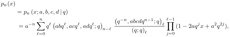
8: 18.28 Askey–Wilson Class

… ►The Askey–Wilson polynomials form a system of OP’s $\{p_n(x)\}$, $n=0,1,2,\mathrm{\dots }$, that are orthogonal with respect to a weight function on a bounded interval, possibly supplemented with discrete weights on a finite set. … ►

18.28.1 $$p_n(x)=p_n(x;a,b,c,d|q)=a^{-n}\sum _{\mathrm{\ell }=0}^n{q}^{\mathrm{\ell }}{(ab{q}^{\mathrm{\ell }},ac{q}^{\mathrm{\ell }},ad{q}^{\mathrm{\ell }};q)}_{n-\mathrm{\ell }}\frac{{(q^{-n},abcd{q}^{n-1};q)}_{\mathrm{\ell }}}{{(q;q)}_{\mathrm{\ell }}}\prod _{j=0}^{\mathrm{\ell }-1}(1-2a{q}^{j}x+a^2{q}^{2j}),$$

ⓘ

Defines:

$p_n(x;a,b,c,d|q)$: Askey–Wilson polynomial

Symbols:

${(a;q)}_n$: $q$-Pochhammer symbol (or $q$-shifted factorial), ${(a_1,a_2,\mathrm{\dots },a_r;q)}_n$: multiple $q$-Pochhammer symbol, $p_n(x)$: polynomial of degree $n$ , $q$: real variable, $\mathrm{\ell }$: nonnegative integer, $n$: nonnegative integer and $x$: real variable

Referenced by:

(18.28.29), §18.28(ii), §18.38(iii), Erratum (V1.2.0) for Equation (18.28.1)

Permalink:

http://dlmf.nist.gov/18.28.E1

Encodings:

pMML, png, TeX

See also:

Annotations for §18.28(ii), §18.28 and Ch.18

… ►Also, $x_{\mathrm{\ell }}$ are the points $\frac{1}{2}(\alpha q^{\mathrm{\ell }}+{\alpha }^{-1}{q}^{-\mathrm{\ell }})$ with $\alpha$ any of the $a,b,c,d$ whose absolute value exceeds $1$, and the sum is over the $\mathrm{\ell }=0,1,2,\mathrm{\dots }$ with $|\alpha q^{\mathrm{\ell }}|>1$. … ►

18.28.7 $$Q_n(\cos \theta ;a,b|q)=p_n(\cos \theta ;a,b,0,0|q)=a^{-n}\sum _{\mathrm{\ell }=0}^n{q}^{\mathrm{\ell }}\frac{{(ab{q}^{\mathrm{\ell }};q)}_{n-\mathrm{\ell }}{(q^{-n};q)}_{\mathrm{\ell }}}{{(q;q)}_{\mathrm{\ell }}}\prod _{j=0}^{\mathrm{\ell }-1}(1-2a{q}^j\cos \theta +a^2{q}^{2j})=\frac{{(ab;q)}_n}{a^n}{}_3{}^{}\varphi _2^{}(\genfrac{}{}{0pt}{}{q^{-n},a{\mathrm{e}}^{\mathrm{i}\theta },a{\mathrm{e}}^{-\mathrm{i}\theta }}{ab,0};q,q)={(b{\mathrm{e}}^{-\mathrm{i}\theta };q)}_n{\mathrm{e}}^{\mathrm{i}n\theta }{}_2{}^{}\varphi _1^{}(\genfrac{}{}{0pt}{}{q^{-n},a{\mathrm{e}}^{\mathrm{i}\theta }}{b^{-1}{q}^{1-n}{\mathrm{e}}^{\mathrm{i}\theta }};q,b^{-1}q{\mathrm{e}}^{-\mathrm{i}\theta }).$$

ⓘ

Defines:

$Q_n(x;a,b|q)$: Al-Salam–Chihara polynomial

Symbols:

$p_n(x;a,b,c,d|q)$: Askey–Wilson polynomial, $\cos z$: cosine function, $\mathrm{e}$: base of natural logarithm, $\mathrm{i}$: imaginary unit, ${(a;q)}_n$: $q$-Pochhammer symbol (or $q$-shifted factorial), ${}_{r+1}{}^{}\varphi _s^{}(a_0,\mathrm{\dots },a_r;b_1,\mathrm{\dots },b_s;q,z)$ or ${}_{r+1}{}^{}\varphi _s^{}(\genfrac{}{}{0pt}{}{a_0,\mathrm{\dots },a_r}{b_1,\mathrm{\dots },b_s};q,z)$: basic hypergeometric (or $q$-hypergeometric) function, $q$: real variable, $\mathrm{\ell }$: nonnegative integer, $n$: nonnegative integer and $x$: real variable

Permalink:

http://dlmf.nist.gov/18.28.E7

Encodings:

pMML, png, TeX

See also:

Annotations for §18.28(iii), §18.28 and Ch.18

… ►Leonard (1982) classified all (finite or infinite) discrete systems of OP’s $p_n(x)$ on a set $\{x(m)\}$ for which there is a system of discrete OP’s $q_m(y)$ on a set $\{y(n)\}$ such that $p_n(x(m))=q_m(y(n))$. …

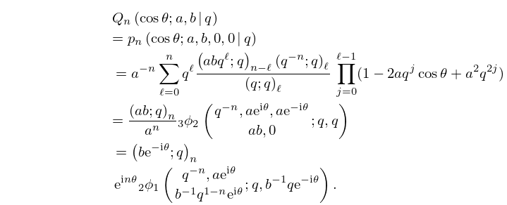
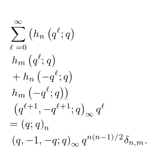
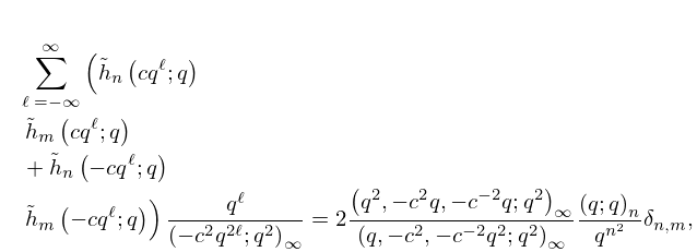
9: 18.27 $q$-Hahn Class

… ►Here $a,b$ are fixed positive real numbers, and $I_{+}$ and $I_{-}$ are sequences of successive integers, finite or unbounded in one direction, or unbounded in both directions. … ►

18.27.4 $$\sum _{y=0}^N{Q}_n(q^{-y})Q_m(q^{-y}){\left[\genfrac{}{}{0.0pt}{}{N}{y}\right]}_q\frac{{(\alpha q;q)}_y{(\beta q;q)}_{N-y}}{{\left(\alpha q\right)}^y}=h_n{\delta }_{n,m},$$ $n,m=0,1,\mathrm{\dots },N$,

ⓘ

Symbols:

${\delta }_{j,k}$: Kronecker delta, ${(a;q)}_n$: $q$-Pochhammer symbol (or $q$-shifted factorial), ${\left[\genfrac{}{}{0.0pt}{}{n}{m}\right]}_q$: $q$-binomial coefficient (or Gaussian polynomial), $y$: real variable, $N$: positive integer, $q$: real variable, $m$: nonnegative integer, $n$: nonnegative integer and $h_n$

Notes:

This is Ismail (2009, (18.5.2)) but the presentation has been simplified.

Referenced by:

§18.27(ii), Erratum (V1.2.0) for Equation (18.27.4)

Permalink:

http://dlmf.nist.gov/18.27.E4

Encodings:

pMML, png, TeX

Correction (effective with 1.1.2):

$q$-Pochhammer symbols now link to their definition.

See also:

Annotations for §18.27(ii), §18.27 and Ch.18

… ►

18.27.14 $$\sum _{y=0}^{\mathrm{\infty }}{p}_n(q^y)p_m(q^y)\frac{{(bq;q)}_y{(aq)}^y}{{(q;q)}_y}=h_n{\delta }_{n,m},$$ ,

ⓘ

Symbols:

${\delta }_{j,k}$: Kronecker delta, ${(a;q)}_n$: $q$-Pochhammer symbol (or $q$-shifted factorial), $y$: real variable, $p_n(x)$: polynomial of degree $n$ , $q$: real variable, $m$: nonnegative integer, $n$: nonnegative integer and $h_n$

Permalink:

http://dlmf.nist.gov/18.27.E14

Encodings:

pMML, png, TeX

See also:

Annotations for §18.27(iv), §18.27 and Ch.18

… ►

18.27.22 $$\sum _{\mathrm{\ell }=0}^{\mathrm{\infty }}\left(h_n(q^{\mathrm{\ell }};q)h_m(q^{\mathrm{\ell }};q)+h_n(-q^{\mathrm{\ell }};q)h_m(-q^{\mathrm{\ell }};q)\right){(q^{\mathrm{\ell }+1},-q^{\mathrm{\ell }+1};q)}_{\mathrm{\infty }}{q}^{\mathrm{\ell }}={(q;q)}_n{(q,-1,-q;q)}_{\mathrm{\infty }}{q}^{n(n-1)/2}{\delta }_{n,m}.$$

ⓘ

Symbols:

${\delta }_{j,k}$: Kronecker delta, $h_n(x;q)$: discrete $q$-Hermite I polynomial, ${(a;q)}_n$: $q$-Pochhammer symbol (or $q$-shifted factorial), ${(a_1,a_2,\mathrm{\dots },a_r;q)}_n$: multiple $q$-Pochhammer symbol, $q$: real variable, $\mathrm{\ell }$: nonnegative integer, $m$: nonnegative integer and $n$: nonnegative integer

Permalink:

http://dlmf.nist.gov/18.27.E22

Encodings:

pMML, png, TeX

See also:

Annotations for §18.27(vii), §18.27(vii), §18.27 and Ch.18

… ►

18.27.24 $$\sum _{\mathrm{\ell }=-\mathrm{\infty }}^{\mathrm{\infty }}\left({\tilde{h}}_n(c{q}^{\mathrm{\ell }};q){\tilde{h}}_m(c{q}^{\mathrm{\ell }};q)+{\tilde{h}}_n(-c{q}^{\mathrm{\ell }};q){\tilde{h}}_m(-c{q}^{\mathrm{\ell }};q)\right)\frac{q^{\mathrm{\ell }}}{{(-c^2{q}^{2\mathrm{\ell }};q^2)}_{\mathrm{\infty }}}=2\frac{{(q^2,-c^{2}q,-c^{-2}q;q^2)}_{\mathrm{\infty }}}{{(q,-c^2,-c^{-2}{q}^2;q^2)}_{\mathrm{\infty }}}\frac{{(q;q)}_n}{q^{n^2}}{\delta }_{n,m},$$ $c>0$.

ⓘ

Symbols:

${\delta }_{j,k}$: Kronecker delta, ${\tilde{h}}_n(x;q)$: discrete $q$-Hermite II polynomial, ${(a;q)}_n$: $q$-Pochhammer symbol (or $q$-shifted factorial), ${(a_1,a_2,\mathrm{\dots },a_r;q)}_n$: multiple $q$-Pochhammer symbol, $q$: real variable, $\mathrm{\ell }$: nonnegative integer, $m$: nonnegative integer and $n$: nonnegative integer

Permalink:

http://dlmf.nist.gov/18.27.E24

Encodings:

pMML, png, TeX

See also:

Annotations for §18.27(vii), §18.27(vii), §18.27 and Ch.18

…

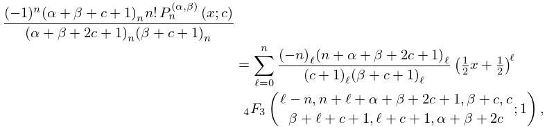
10: 18.30 Associated OP’s

… ►

18.30.5 $$\frac{{(-1)}^n{\left(\alpha +\beta +c+1\right)}_{n}n!P_n^{(\alpha ,\beta )}(x;c)}{{\left(\alpha +\beta +2c+1\right)}_n{\left(\beta +c+1\right)}_n}=\sum _{\mathrm{\ell }=0}^n\frac{{\left(-n\right)}_{\mathrm{\ell }}{\left(n+\alpha +\beta +2c+1\right)}_{\mathrm{\ell }}}{{\left(c+1\right)}_{\mathrm{\ell }}{\left(\beta +c+1\right)}_{\mathrm{\ell }}}{\left(\frac{1}{2}x+\frac{1}{2}\right)}^{\mathrm{\ell }}{}_4{}^{}F_3^{}(\genfrac{}{}{0pt}{}{\mathrm{\ell }-n,n+\mathrm{\ell }+\alpha +\beta +2c+1,\beta +c,c}{\beta +\mathrm{\ell }+c+1,\mathrm{\ell }+c+1,\alpha +\beta +2c};1),$$

ⓘ

Symbols:

${}_p{}^{}F_q^{}(a_1,\mathrm{\dots },a_p;b_1,\mathrm{\dots },b_q;z)$ or ${}_p{}^{}F_q^{}(\genfrac{}{}{0pt}{}{a_1,\mathrm{\dots },a_p}{b_1,\mathrm{\dots },b_q};z)$: alternatively ${}_p{}^{}F_q^{}(𝐚;𝐛;z)$ or ${}_p{}^{}F_q^{}(\genfrac{}{}{0pt}{}{𝐚}{𝐛};z)$
generalized hypergeometric function, ${\left(a\right)}_n$: Pochhammer’s symbol (or shifted factorial), $P_n^{(\alpha ,\beta )}(x;c)$: associated Jacobi polynomial, $!$: factorial (as in $n!$), $\mathrm{\ell }$: nonnegative integer, $n$: nonnegative integer and $x$: real variable

Referenced by:

§18.30

Permalink:

http://dlmf.nist.gov/18.30.E5

Encodings:

pMML, png, TeX

See also:

Annotations for §18.30(i), §18.30 and Ch.18

►where the generalized hypergeometric function ${}_4{}^{}F_3^{}$ is defined by (16.2.1). … ►For other cases there may also be, in addition to a possible integral as in (18.30.10), a finite sum of discrete weights on the negative real $x$-axis each multiplied by the polynomial product evaluated at the corresponding values of $x$, as in (18.2.3). … ►They can be expressed in terms of type 3 Pollaczek polynomials (which are also associated type 2 Pollaczek polynomials) by (18.35.10). … ►The type 3 Pollaczek polynomials are the associated type 2 Pollaczek polynomials, see §18.35. …