exceptional values

SearchAdvancedHelp

(0.002 seconds)

41—50 of 55 matching pages

41: Mathematical Introduction

… ►With a few exceptions the adopted notations are the same as those in standard applied mathematics and physics literature. ►The exceptions are ones for which the existing notations have drawbacks. … ►With two real variables, special functions are depicted as 3D surfaces, with vertical height corresponding to the value of the function, and coloring added to emphasize the 3D nature. … ►Special functions with a complex variable are depicted as colored 3D surfaces in a similar way to functions of two real variables, but with the vertical height corresponding to the modulus (absolute value) of the function. … ►05, and the corresponding function values are tabulated to 8 decimal places or 8 significant figures. …

42: Bibliography N

… ►

Tables Relating to Mathieu Functions: Characteristic Values, Coefficients, and Joining Factors. 2nd edition, National Bureau of Standards Applied Mathematics Series, U.S. Government Printing Office, Washington, D.C..

ⓘ

External Links:

MathReview, ZentralBlatt

Referenced by:

§28.1, §28.26(i), 6th item, Notations S, Notations S.

Encodings:

BibTeX

… ►

Coulomb Functions for Large Values of the Parameter $\eta$ . Technical report Atomic Energy of Canada Limited, Chalk River, Ontario.

ⓘ

Notes:

Rep. CRT-526

External Links:

MathReview (A. Erdélyi)

Referenced by:

§33.7.

Encodings:

BibTeX

… ►

Die Gammafunktion. Band I. Handbuch der Theorie der Gammafunktion. Band II. Theorie des Integrallogarithmus und verwandter Transzendenten. Chelsea Publishing Co., New York (German).

ⓘ

Notes:

Both books are textually unaltered except for correction of errata.

External Links:

MathReview

Referenced by:

N. Nielsen (1906a), N. Nielsen (1906b).

Encodings:

BibTeX

…

43: 19.1 Special Notation

… ►All square roots have their principal values. … ►The functions (19.1.1) and (19.1.2) are used in Erdélyi et al. (1953b, Chapter 13), except that $\mathrm{\Pi }({\alpha }^2,k)$ and $\mathrm{\Pi }(\varphi ,{\alpha }^2,k)$ are denoted by ${\mathrm{\Pi }}_1(\nu ,k)$ and $\mathrm{\Pi }(\varphi ,\nu ,k)$, respectively, where $\nu =-{\alpha }^2$. …

44: 32.2 Differential Equations

… ►be a nonlinear second-order differential equation in which $F$ is a rational function of $w$ and $dw/dz$, and is locally analytic in $z$, that is, analytic except for isolated singularities in $ℂ$. … ►For arbitrary values of the parameters $\alpha$, $\beta$, $\gamma$, and $\delta$, the general solutions of ${\text{P}}_{\text{I}}$–${\text{P}}_{\text{VI}}$ are transcendental, that is, they cannot be expressed in closed-form elementary functions. However, for special values of the parameters, equations ${\text{P}}_{\text{II}}$–${\text{P}}_{\text{VI}}$ have special solutions in terms of elementary functions, or special functions defined elsewhere in the DLMF. …

45: 1.8 Fourier Series

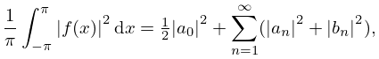
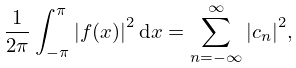
… ►Formally, if $f(x)$ is a real- or complex-valued $2\pi$-periodic function, … ►

1.8.5 $$\frac{1}{\pi }{\int }_{-\pi }^{\pi }{\left|f(x)\right|}^{2}dx=\frac{1}{2}{\left|a_0\right|}^2+\sum _{n=1}^{\mathrm{\infty }}({\left|a_n\right|}^2+{\left|b_n\right|}^2),$$

ⓘ

Symbols:

$\pi$: the ratio of the circumference of a circle to its diameter, $dx$: differential of $x$ , $\int$: integral, $n$: nonnegative integer and $\left|x\right|$: absolute value of $x$

Referenced by:

Erratum (V1.2.0) for Equations (1.8.5), (1.8.6)

Permalink:

http://dlmf.nist.gov/1.8.E5

Encodings:

pMML, png, TeX

Modification (effective with 1.2.0):

Previously this equation was given as an inequality. For square integrable functions this inequality $\ge$ can be sharpened to $=$.

See also:

Annotations for §1.8(i), §1.8(i), §1.8 and Ch.1

►

1.8.6 $$\frac{1}{2\pi }{\int }_{-\pi }^{\pi }{\left|f(x)\right|}^{2}dx=\sum _{n=-\mathrm{\infty }}^{\mathrm{\infty }}{\left|c_n\right|}^2,$$

ⓘ

Symbols:

$\pi$: the ratio of the circumference of a circle to its diameter, $dx$: differential of $x$ , $\int$: integral, $n$: nonnegative integer and $\left|x\right|$: absolute value of $x$

Referenced by:

§1.8(i), Erratum (V1.2.0) for Equations (1.8.5), (1.8.6)

Permalink:

http://dlmf.nist.gov/1.8.E6

Encodings:

pMML, png, TeX

Modification (effective with 1.2.0):

Previously this equation was given as an inequality. For square integrable functions this inequality $\ge$ can be sharpened to $=$.

See also:

Annotations for §1.8(i), §1.8(i), §1.8 and Ch.1

… ►

1.8.8 $$L_n=\frac{1}{\pi }{\int }_0^{\pi }\frac{\left|\sin \left(n+\frac{1}{2}\right)t\right|}{\sin \left(\frac{1}{2}t\right)}dt,$$ $n=0,1,\mathrm{\dots }$.

ⓘ

Defines:

$L_n$: Lebesgue constants (locally)

Symbols:

$\pi$: the ratio of the circumference of a circle to its diameter, $dx$: differential of $x$ , $\int$: integral, $\sin z$: sine function, $n$: nonnegative integer and $\left|x\right|$: absolute value of $x$

Permalink:

http://dlmf.nist.gov/1.8.E8

Encodings:

pMML, png, TeX

See also:

Annotations for §1.8(i), §1.8(i), §1.8 and Ch.1

… ►Let $f(x)$ be an absolutely integrable function of period $2\pi$, and continuous except at a finite number of points in any bounded interval. …

46: 28.29 Definitions and Basic Properties

… ► $Q(z)$ is either a continuous and real-valued function for $z\in ℝ$ or an analytic function of $z$ in a doubly-infinite open strip that contains the real axis. … ►The solutions of period $\pi$ or $2\pi$ are exceptional in the following sense. … ► $Q(x)$ is assumed to be real-valued throughout this subsection. … ►Conversely, for a given $\lambda$, the value of $△(\lambda )$ is needed for the computation of $\nu$. …

47: 33.14 Definitions and Basic Properties

… ►For nonzero values of $ϵ$ and $r$ the function $h(ϵ,\mathrm{\ell };r)$ is defined by … ► $h(ϵ,\mathrm{\ell };r)$ is real and an analytic function of each of $r$ and $ϵ$ in the intervals and , except when $r=0$ or $ϵ=0$. …

48: Errata

… ►We also discuss non-classical Laguerre polynomials and give much more details and examples on exceptional orthogonal polynomials. … ►

The constraints in (14.5.3), (14.5.4) on $\nu +\mu$ have been corrected to exclude all negative integers since the Ferrers function of the second kind is not defined for these values.

Reported by Hans Volkmer on 2021-06-02

… ►

The asymptotic results were originally for $\nu$ real valued and $\nu \to +\mathrm{\infty }$. However, these results are also valid for complex values of $\nu$. The maximum sectors of validity are now specified.

… ►

The Olver hypergeometric function $𝐅(a,b;c;z)$, previously omitted from the left-hand sides to make the formulas more concise, has been added. In Equations (15.6.1)–(15.6.5), (15.6.7)–(15.6.9), the constraint has been added. In (15.6.6), the constraint has been added. In Section 15.6 Integral Representations, the sentence immediately following (15.6.9), “These representations are valid when , except (15.6.6) which holds for .”, has been removed.

… ►

In the line just below (18.15.4), it was previously stated “is less than twice the first neglected term in absolute value.” It now states “is less than twice the first neglected term in absolute value, in which one has to take $\cos {\theta }_{n,m,\mathrm{\ell }}=1$.”

Reported by Gergő Nemes on 2019-02-08

…

49: Bibliography M

… ►

Connection between quantum systems involving the fourth Painlevé transcendent and $k$-step rational extensions of the harmonic oscillator related to Hermite exceptional orthogonal polynomial. J. Math. Phys. 57 (5), pp. Paper 052101, 15 pp..

ⓘ

External Links:

ISSN 0022-2488, Document, Link, MathReview Entry

Referenced by:

§18.38(iii).

Encodings:

BibTeX

… ►

Exceptional orthogonal polynomials.

ⓘ

Notes:

Lecture at ICMAT School on Orthogonal Polynomials in Approximation Theory and Mathematical Physics, available at https://www.icmat.es/RT/optrim/school/lectures/Milson/icmat17.pdf

Referenced by:

§18.36(vi), §18.38(iii).

Encodings:

BibTeX

… ►

CODATA recommended values of the fundamental physical constants: 2002. Rev. Mod.Phys. 77, pp. 1–107.

ⓘ

Referenced by:

§18.39(ii).

Encodings:

BibTeX

…

50: 18.36 Miscellaneous Polynomials

… ►

§18.36(vi) Exceptional Orthogonal Polynomials

… ►The exceptional type III $X_m$-EOP’s are missing orders $1,\mathrm{\dots },m$. … ►The resulting EOP’s, ${\widehat{L}}_n^{(k)}\left(x\right)$, $n=1,2,\mathrm{\dots }$ satisfy … ►The $y(x)={\widehat{L}}_n^{(k)}\left(x\right)$ satisfy a second order Sturm–Liouville eigenvalue problem of the type illustrated in Table 18.8.1, as satisfied by classical OP’s, but now with rational, rather than polynomial coefficients: … ►The type III $X_2$-Hermite EOP’s, missing polynomial orders $1$ and $2$, are the complete set of polynomials, with real coefficients and defined explicitly as …