even%20part

(0.001 seconds)

11—20 of 399 matching pages

11: 18.32 OP’s with Respect to Freud Weights

… ►where

Q(x)

is real, even, nonnegative, and continuously differentiable, where

xQ^{\prime}(x)

increases for

x>0

, and

Q^{\prime}(x)\to\infty

x\to\infty

, see Freud (1969). …See the early survey by Nevai (1986, Part 2). …

12: Bibliography K

… ►

P. L. Kapitsa (1951b) The computation of the sums of negative even powers of roots of Bessel functions. Doklady Akad. Nauk SSSR (N.S.) 77, pp. 561–564.

ⓘ

External Links:: MathReview (A. Erdélyi), ZentralBlatt
Referenced by:: §10.21(xiii).
Encodings:: BibTeX

… ►

R. B. Kearfott, M. Dawande, K. Du, and C. Hu (1994) Algorithm 737: INTLIB: A portable Fortran 77 interval standard-function library. ACM Trans. Math. Software 20 (4), pp. 447–459.

ⓘ

External Links:: ISSN 0098-3500, Document, GAMS (module 737; package TOMS), ZentralBlatt
Referenced by:: 1st item.
Encodings:: BibTeX

… ►

M. K. Kerimov (1980) Methods of computing the Riemann zeta-function and some generalizations of it. USSR Comput. Math. and Math. Phys. 20 (6), pp. 212–230.

ⓘ

External Links:: Document, MathReview (Matti Jutila), ZentralBlatt
Referenced by:: §25.18(i).
Encodings:: BibTeX

… ►

A. V. Kitaev and A. H. Vartanian (2004) Connection formulae for asymptotics of solutions of the degenerate third Painlevé equation. I. Inverse Problems 20 (4), pp. 1165–1206.

ⓘ

External Links:: ISSN 0266-5611, Document, MathReview (Shun Shimomura), ZentralBlatt
Referenced by:: §32.11(iv).
Encodings:: BibTeX

… ►

T. H. Koornwinder (2009) The Askey scheme as a four-manifold with corners. Ramanujan J. 20 (3), pp. 409–439.

ⓘ

External Links:: ISSN 1382-4090, Document, FullText, MathReview (José Luis López), ZentralBlatt
Referenced by:: §18.26(v), §18.26(v).
Encodings:: BibTeX

…

13: 36.2 Catastrophes and Canonical Integrals

… ►

36.2.15

\Psi_{K}\left(\boldsymbol{{0}}\right)=\frac{2}{K+2}\Gamma\left(\frac{1}{K+2}% \right)\*\begin{cases}\exp\left(i\dfrac{\pi}{2(K+2)}\right),&K\text{ even,}\\ \cos\left(\dfrac{\pi}{2(K+2)}\right),&K\text{ odd}.\end{cases}

ⓘ

Symbols:: $\Gamma\left(\NVar{z}\right)$ : gamma function, $\Psi_{\NVar{K}}\left(\NVar{\mathbf{x}}\right)$ : canonical integral function, $\pi$ : the ratio of the circumference of a circle to its diameter, $\cos\NVar{z}$ : cosine function, $\exp\NVar{z}$ : exponential function, $\mathrm{i}$ : imaginary unit and $K$ : codimension
Referenced by:: §36.2(ii)
Permalink:: http://dlmf.nist.gov/36.2.E15
Encodings:: pMML, png, TeX
See also:: Annotations for §36.2(ii), §36.2 and Ch.36

… ►

\frac{{\partial}^{2q+1}}{{\partial x_{1}}^{2q+1}}\Psi_{K}\left(\boldsymbol{{0}% }\right)=0,

K

even,

►

\frac{{\partial}^{2q}}{{\partial x_{1}}^{2q}}\Psi_{K}\left(\boldsymbol{{0}}% \right)=\frac{2}{K+2}\Gamma\left(\frac{2q+1}{K+2}\right)\exp\left(i\frac{\pi}{% 2}\left(\frac{2q+1}{K+2}+2q\right)\right),

K

even.

… ►

36.2.20

\Psi^{(\mathrm{E})}\left(x,y,0\right)=2\pi^{2}(\tfrac{2}{3})^{2/3}\Re\left(% \operatorname{Ai}\left(\frac{x+iy}{12^{1/3}}\right)\operatorname{Bi}\left(% \frac{x-iy}{12^{1/3}}\right)\right),

ⓘ

Symbols:: $\operatorname{Ai}\left(\NVar{z}\right)$ : Airy function, $\operatorname{Bi}\left(\NVar{z}\right)$ : Airy function, $\pi$ : the ratio of the circumference of a circle to its diameter, $\Psi^{(\mathrm{E})}\left(\NVar{\mathbf{x}}\right)$ : elliptic umbilic canonical integral function, $\mathrm{i}$ : imaginary unit, $\Re$ : real part, $y$ : real parameter and $x$ : real parameter
Referenced by:: §36.2(ii), §36.7(iii), §36.8
Permalink:: http://dlmf.nist.gov/36.2.E20
Encodings:: pMML, png, TeX
See also:: Annotations for §36.2(ii), §36.2 and Ch.36

… ►

36.2.29

\Psi^{(\mathrm{H})}\left(0,0,z\right)=\overline{\Psi^{(\mathrm{H})}\left(0,0,-% z\right)}=\frac{2^{1/3}}{\sqrt{3}}\exp\left(\frac{1}{27}iz^{3}\right)\Psi^{(% \mathrm{E})}\left(0,0,-\frac{z}{2^{2/3}}\right),

-\infty<z<\infty

ⓘ

Symbols:: $\overline{\NVar{z}}$ : complex conjugate, $\Psi^{(\mathrm{E})}\left(\NVar{\mathbf{x}}\right)$ : elliptic umbilic canonical integral function, $\exp\NVar{z}$ : exponential function, $\Psi^{(\mathrm{H})}\left(\NVar{\mathbf{x}}\right)$ : hyperbolic umbilic canonical integral function, $\mathrm{i}$ : imaginary unit and $z$ : real parameter
Referenced by:: Erratum (V1.0.5) for Chapters 8, 20, 36
Permalink:: http://dlmf.nist.gov/36.2.E29
Encodings:: pMML, png, TeX
Addition (effective with 1.0.5):: This equation has been added. For the proof see Berry and Howls (2010).
See also:: Annotations for §36.2(iv), §36.2 and Ch.36

14: 20.1 Special Notation

… ► ►►►►

$m$ , $n$	integers.
…
$\tau$ $(\in\mathbb{C})$	the lattice parameter, $\Im\tau>0$ .
$q$ $(\in\mathbb{C})$	the nome, $q=e^{i\pi\tau}$ , $0<\left\|q\right\|<1$ . Since $\tau$ is not a single-valued function of $q$ , it is assumed that $\tau$ is known, even when $q$ is specified. Most applications concern the rectangular case $\Re\tau=0$ , $\Im\tau>0$ , so that $0<q<1$ and $\tau$ and $q$ are uniquely related.
…

… ►When

\tau

is fixed the notation is often abbreviated in the literature as

\theta_{j}(z)

, or even as simply

\theta_{j}

, it being then understood that the argument is the primary variable. …

Zhang and Jin (1996, pp. 652, 689) includes $\operatorname{Si}\left(x\right)$ , $\operatorname{Ci}\left(x\right)$ , $x=0(.5)20(2)30$ , 8D; $\operatorname{Ei}\left(x\right)$ , $E_{1}\left(x\right)$ , $x=[0,100]$ , 8S.

… ►

•

Abramowitz and Stegun (1964, Chapter 5) includes the real and imaginary parts of $ze^{z}E_{1}\left(z\right)$ , $x=-19(1)20$ , $y=0(1)20$ , 6D; $e^{z}E_{1}\left(z\right)$ , $x=-4(.5)-2$ , $y=0(.2)1$ , 6D; $E_{1}\left(z\right)+\ln z$ , $x=-2(.5)2.5$ , $y=0(.2)1$ , 6D.

►

•

Zhang and Jin (1996, pp. 690–692) includes the real and imaginary parts of $E_{1}\left(z\right)$ , $\pm x=0.5,1,3,5,10,15,20,50,100$ , $y=0(.5)1(1)5(5)30,50,100$ , 8S.

16: Bibliography G

… ►

B. Gabutti and B. Minetti (1981) A new application of the discrete Laguerre polynomials in the numerical evaluation of the Hankel transform of a strongly decreasing even function. J. Comput. Phys. 42 (2), pp. 277–287.

ⓘ

External Links:: Document, ZentralBlatt
Referenced by:: §10.74(vii).
Encodings:: BibTeX

… ►

W. Gautschi (1994) Algorithm 726: ORTHPOL — a package of routines for generating orthogonal polynomials and Gauss-type quadrature rules. ACM Trans. Math. Software 20 (1), pp. 21–62.

ⓘ

Notes:: For remark see same journal 24(1998), p. 355.
External Links:: Document, ISSN 0098-3500, GAMS (module 726; package TOMS), ZentralBlatt
Referenced by:: 2nd item, §3.5(v), §3.5(v).
Encodings:: BibTeX

… ►

M. Geller and E. W. Ng (1971) A table of integrals of the error function. II. Additions and corrections. J. Res. Nat. Bur. Standards Sect. B 75B, pp. 149–163.

ⓘ

Notes:: See for the first part same journal, Sect. B 73, 1-20 (1969)
External Links:: MathReview, ZentralBlatt
Referenced by:: §7.14(iii).
Encodings:: BibTeX

… ►

A. Gil, J. Segura, and N. M. Temme (2014) Algorithm 939: computation of the Marcum Q-function. ACM Trans. Math. Softw. 40 (3), pp. 20:1–20:21.

ⓘ

Notes:: Includes Fortran program claiming 12S accuracy
External Links:: ISSN 0098-3500, Link, Document, MathReview Entry, ZentralBlatt
Referenced by:: 3rd item, §10.77(ix).
Encodings:: BibTeX

… ►

Ya. I. Granovskiĭ, I. M. Lutzenko, and A. S. Zhedanov (1992) Mutual integrability, quadratic algebras, and dynamical symmetry. Ann. Phys. 217 (1), pp. 1–20.

ⓘ

External Links:: ISSN 0003-4916, Link, MathReview (A. O. Barut), ZentralBlatt
Referenced by:: §18.38(iii).
Encodings:: BibTeX

…

17: 2.11 Remainder Terms; Stokes Phenomenon

… ►Even when the series converges this is unwise: the tail needs to be majorized rigorously before the result can be guaranteed. For divergent expansions the situation is even more difficult. … ►If we permit the use of nonelementary functions as approximants, then even more powerful re-expansions become available. … ►That the change in their forms is discontinuous, even though the function being approximated is analytic, is an example of the Stokes phenomenon. … ►For example, using double precision

d_{20}

is found to agree with (2.11.31) to 13D. …

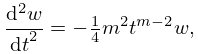
18: 9.13 Generalized Airy Functions

… ►

9.13.6

A_{n}\left(-z\right)=\begin{cases}pz^{1/2}\left(J_{-p}\left(\zeta\right)+J_{p}% \left(\zeta\right)\right),&n\text{ odd},\\ p^{1/2}B_{n}\left(z\right),&n\text{ even},\end{cases}

ⓘ

Symbols:: $J_{\NVar{\nu}}\left(\NVar{z}\right)$ : Bessel function of the first kind, $A_{\NVar{n}}\left(\NVar{z}\right)$ : generalized Airy function, $B_{\NVar{n}}\left(\NVar{z}\right)$ : generalized Airy function, $z$ : complex variable, $n$ : parameter, $p$ : variable and $\zeta$ : variable
Source:: Swanson and Headley (1967, (5a)–(5b))
Permalink:: http://dlmf.nist.gov/9.13.E6
Encodings:: pMML, png, TeX
See also:: Annotations for §9.13(i), §9.13 and Ch.9

… ►

9.13.10

A_{n}\left(-z\right)=\begin{cases}2\sqrt{p/\pi}\cos\left(\tfrac{1}{2}p\pi% \right)z^{-n/4}\left(\cos\left(\zeta-\tfrac{1}{4}\pi\right)+e^{|\Im\zeta|}O% \left(\zeta^{-1}\right)\right),&\text{$|\operatorname{ph}z|\leq 2p\pi-\delta$,% $n$ odd},\\ \sqrt{p/\pi}z^{-n/4}e^{\zeta}\left(1+O\left(\zeta^{-1}\right)\right),&\text{$|% \operatorname{ph}z|\leq p\pi-\delta$, $n$ even},\end{cases}

ⓘ

Symbols:: $O\left(\NVar{x}\right)$ : order not exceeding, $A_{\NVar{n}}\left(\NVar{z}\right)$ : generalized Airy function, $\pi$ : the ratio of the circumference of a circle to its diameter, $\cos\NVar{z}$ : cosine function, $\mathrm{e}$ : base of natural logarithm, $\Im$ : imaginary part, $\operatorname{ph}$ : phase, $z$ : complex variable, $\delta$ : small positive constant, $n$ : parameter, $p$ : variable and $\zeta$ : variable
Source:: Swanson and Headley (1967, (14)–(15))
Permalink:: http://dlmf.nist.gov/9.13.E10
Encodings:: pMML, png, TeX
See also:: Annotations for §9.13(i), §9.13 and Ch.9

… ►

9.13.12

B_{n}\left(-z\right)=\begin{cases}-(\ifrac{2}{\sqrt{\pi}})\sin\left(\tfrac{1}{% 2}p\pi\right)z^{-n/4}\left(\sin\left(\zeta-\tfrac{1}{4}\pi\right)+e^{\left|\Im% \zeta\right|}O\left(\zeta^{-1}\right)\right),&\left|\operatorname{ph}z\right|% \leq 2p\pi-\delta,n\text{ odd},\\ (\ifrac{1}{\sqrt{\pi}})\sin\left(p\pi\right)z^{-n/4}e^{-\zeta}\left(1+O\left(% \zeta^{-1}\right)\right),&\left|\operatorname{ph}z\right|\leq 3p\pi-\delta,n% \text{ even}.\end{cases}

ⓘ

Symbols:: $O\left(\NVar{x}\right)$ : order not exceeding, $B_{\NVar{n}}\left(\NVar{z}\right)$ : generalized Airy function, $\pi$ : the ratio of the circumference of a circle to its diameter, $\mathrm{e}$ : base of natural logarithm, $\Im$ : imaginary part, $\operatorname{ph}$ : phase, $\sin\NVar{z}$ : sine function, $z$ : complex variable, $\delta$ : small positive constant, $n$ : parameter, $p$ : variable and $\zeta$ : variable
Source:: Swanson and Headley (1967, (17)–(18))
Permalink:: http://dlmf.nist.gov/9.13.E12
Encodings:: pMML, png, TeX
See also:: Annotations for §9.13(i), §9.13 and Ch.9

… ►where

m=3,4,5,\ldots.

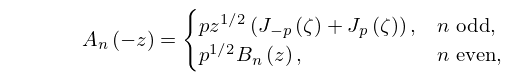
For real variables the solutions of (9.13.13) are denoted by

U_{m}(t)

U_{m}(-t)

when

m

is even, and by

V_{m}(t)

\overline{V}_{m}(t)

when

m

is odd. … ►

9.13.17

\frac{{\mathrm{d}}^{2}w}{{\mathrm{d}t}^{2}}=-\tfrac{1}{4}m^{2}t^{m-2}w,

m

even,

ⓘ

Defines:: $W_{m}$ : function (locally)
Symbols:: $\frac{\mathrm{d}\NVar{f}}{\mathrm{d}\NVar{x}}$ : derivative of $f$ with respect to $x$ , $w$ : function and $m$ : index
Source:: Olver (1977a, (2.11), p. 131)
Referenced by:: §9.13(i)
Permalink:: http://dlmf.nist.gov/9.13.E17
Encodings:: pMML, png, TeX
See also:: Annotations for §9.13(i), §9.13 and Ch.9

…

19: 34.10 Zeros

… ►However, the

\mathit{3j}

and

\mathit{6j}

symbols may vanish for certain combinations of the angular momenta and projective quantum numbers even when the triangle conditions are fulfilled. …

20: 35.10 Methods of Computation

… ►These algorithms are extremely efficient, converge rapidly even for large values of

m

, and have complexity linear in

m