elliptic cases of R-a(b;z)

SearchAdvancedHelp

(0.007 seconds)

11—20 of 885 matching pages

11: 22.5 Special Values

… ►Table 22.5.1 gives the value of each of the 12 Jacobian elliptic functions, together with its $z$-derivative (or at a pole, the residue), for values of $z$ that are integer multiples of $K$, $\mathrm{i}{K}^{\prime }$. … ►Table 22.5.2 gives $\mathrm{sn}(z,k)$, $\mathrm{cn}(z,k)$, $\mathrm{dn}(z,k)$ for other special values of $z$. … ►In these cases the elliptic functions degenerate into elementary trigonometric and hyperbolic functions, respectively. … ►For values of $K,K^{\prime }$ when $k^2=\frac{1}{2}$ (lemniscatic case) see §23.5(iii), and for $k^2={\mathrm{e}}^{\mathrm{i}\pi /3}$ (equianharmonic case) see §23.5(v).

12: 22.4 Periods, Poles, and Zeros

… ►

§22.4(i) Distribution

… ► … ► … ►(b) The difference between p and the nearest q is a half-period of $\mathrm{p}\mathrm{q}(z,k)$. … ►For example, $\mathrm{sn}(z+K,k)=\mathrm{cd}(z,k)$. …

13: 19.22 Quadratic Transformations

… ►

Bartky’s Transformation

… ►

§19.22(ii) Gauss’s Arithmetic-Geometric Mean (AGM)

… ►Descending Gauss transformations include, as special cases, transformations of complete integrals into complete integrals; ascending Landen transformations do not. … ►

14: 22.6 Elementary Identities

§22.6 Elementary Identities

… ►

§22.6(ii) Double Argument

… ►

§22.6(iii) Half Argument

… ►

§22.6(iv) Rotation of Argument (Jacobi’s Imaginary Transformation)

… ►See §22.17.

15: 22.18 Mathematical Applications

… ►With $k\in [0,1]$ the mapping $z\to w=\mathrm{sn}(z,k)$ gives a conformal map of the closed rectangle $[-K,K]\times [0,K^{\prime }]$ onto the half-plane $\mathrm{\Im }w\ge 0$, with $0,\pm K,\pm K+\mathrm{i}{K}^{\prime },\mathrm{i}{K}^{\prime }$ mapping to $0,\pm 1,\pm k^{-2},\mathrm{\infty }$ respectively. … ► ►

§22.18(iv) Elliptic Curves and the Jacobi–Abel Addition Theorem

… ►With the identification $x=\mathrm{sn}(z,k)$, $y=d(\mathrm{sn}(z,k))/dz$, the addition law (22.18.8) is transformed into the addition theorem (22.8.1); see Akhiezer (1990, pp. 42, 45, 73–74) and McKean and Moll (1999, §§2.14, 2.16). …

16: 19.15 Advantages of Symmetry

§19.15 Advantages of Symmetry

►Elliptic integrals are special cases of a particular multivariate hypergeometric function called Lauricella’s $F_D$ (Carlson (1961b)). … ► … ►For the many properties of ellipses and triaxial ellipsoids that can be represented by elliptic integrals, any symmetry in the semiaxes remains obvious when symmetric integrals are used (see (19.30.5) and §19.33). …

17: 29.11 Lamé Wave Equation

… ►

29.11.1 $$\frac{d^{2}w}{{dz}^2}+(h-\nu (\nu +1)k^2{\mathrm{sn}}^2(z,k)+k^2{\omega }^2{\mathrm{sn}}^4(z,k))w=0,$$

ⓘ

Symbols:

$\mathrm{sn}(z,k)$: Jacobian elliptic function, $\frac{df}{dx}$: derivative of $f$ with respect to $x$ , $z$: complex variable, $h$: real parameter, $k$: real parameter, $\nu$: real parameter, $\omega$: parameter and $w(z)$: solution

Referenced by:

§29.11, §29.11, §29.18(ii), §29.7(ii)

Permalink:

http://dlmf.nist.gov/29.11.E1

Encodings:

pMML, png, TeX

See also:

Annotations for §29.11 and Ch.29

… ►In the case $\omega =0$, (29.11.1) reduces to Lamé’s equation (29.2.1). ►For properties of the solutions of (29.11.1) see Arscott (1956, 1959), Arscott (1964b, Chapter X), Erdélyi et al. (1955, §16.14), Fedoryuk (1989), and Müller (1966a, b, c).

18: 23.4 Graphics

… ►

§23.4(i) Real Variables

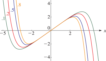
►Line graphs of the Weierstrass functions $\mathrm{\wp }\left(x\right)$, $\zeta \left(x\right)$, and $\sigma \left(x\right)$, illustrating the lemniscatic and equianharmonic cases. … ►

►►

Figure 23.4.6: $\sigma (x;0,g_3)$ for $-5\le x\le 5$, $g_3$ = 0. … Magnify

… ►

§23.4(ii) Complex Variables

►Surfaces for the Weierstrass functions $\mathrm{\wp }\left(z\right)$, $\zeta \left(z\right)$, and $\sigma \left(z\right)$. …

19: 19.13 Integrals of Elliptic Integrals

§19.13 Integrals of Elliptic Integrals

►

§19.13(i) Integration with Respect to the Modulus

… ►Cvijović and Klinowski (1994) contains fractional integrals (with free parameters) for $F(\varphi ,k)$ and $E(\varphi ,k)$, together with special cases. ►

§19.13(iii) Laplace Transforms

►For direct and inverse Laplace transforms for the complete elliptic integrals $K\left(k\right)$, $E\left(k\right)$, and $D\left(k\right)$ see Prudnikov et al. (1992a, §3.31) and Prudnikov et al. (1992b, §§3.29 and 4.3.33), respectively.

20: 19.7 Connection Formulas

§19.7 Connection Formulas

… ►

Reciprocal-Modulus Transformation

… ►

Imaginary-Modulus Transformation

… ►

§19.7(iii) Change of Parameter of $\mathrm{\Pi }(\varphi ,{\alpha }^2,k)$

… ►The first of the three relations maps each circular region onto itself and each hyperbolic region onto the other; in particular, it gives the Cauchy principal value of $\mathrm{\Pi }(\varphi ,{\alpha }^2,k)$ when ${\alpha }^2>{\csc }^2\varphi$ (see (19.6.5) for the complete case). …