divided differences

SearchAdvancedHelp

(0.005 seconds)

1—10 of 130 matching pages

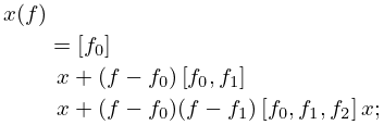
1: 3.3 Interpolation

… ►

§3.3(iii) Divided Differences

… ►

$$\left[z_0\right]f=f_0,$$

►

$$\left[z_0,z_1\right]f=(\left[z_1\right]f-\left[z_0\right]f)/(z_1-z_0),$$

►

$$\left[z_0,z_1,z_2\right]f=(\left[z_1,z_2\right]f-\left[z_0,z_1\right]f)/(z_2-z_0),$$

… ►

3.3.39 $$x(f)=\left[f_0\right]x+(f-f_0)\left[f_0,f_1\right]x+(f-f_0)(f-f_1)\left[f_0,f_1,f_2\right]x;$$

ⓘ

Symbols:

$\left[z_0,z_1,\mathrm{\dots },z_n\right]f$: divided difference, $f(z)$: function and $f_t$: function values

Permalink:

http://dlmf.nist.gov/3.3.E39

Encodings:

pMML, png, TeX

See also:

Annotations for §3.3(v), §3.3(v), §3.3 and Ch.3

…

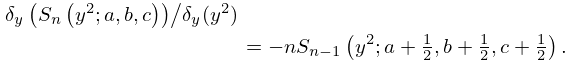
2: 18.26 Wilson Class: Continued

… ►

18.26.14 $${\delta }_y\left(W_n(y^2;a,b,c,d)\right)/{\delta }_y(y^2)=-n(n+a+b+c+d-1)W_{n-1}(y^2;a+\frac{1}{2},b+\frac{1}{2},c+\frac{1}{2},d+\frac{1}{2}).$$

ⓘ

Symbols:

$W_n(x;a,b,c,d)$: Wilson polynomial, ${\delta }_x$: central difference, $y$: real variable and $n$: nonnegative integer

Referenced by:

§16.4(iii), §18.26(iii)

Permalink:

http://dlmf.nist.gov/18.26.E14

Encodings:

pMML, png, TeX

See also:

Annotations for §18.26(iii), §18.26 and Ch.18

►

18.26.15 $${\delta }_y\left(S_n(y^2;a,b,c)\right)/{\delta }_y(y^2)=-n{S}_{n-1}(y^2;a+\frac{1}{2},b+\frac{1}{2},c+\frac{1}{2}).$$

ⓘ

Symbols:

${\delta }_x$: central difference, $S_n(x;a,b,c)$: continuous dual Hahn polynomial, $y$: real variable and $n$: nonnegative integer

Permalink:

http://dlmf.nist.gov/18.26.E15

Encodings:

pMML, png, TeX

See also:

Annotations for §18.26(iii), §18.26 and Ch.18

…

3: 21.7 Riemann Surfaces

… ►

21.7.15 $$4{𝜼}^1(T)\cdot {𝜼}^2(T)=\frac{1}{2}\left(|T\ominus U|-g-1\right)(mod2),$$

ⓘ

Symbols:

$g$: positive integer, $U$: subset of $B$ and $T$: subset of $B$

Permalink:

http://dlmf.nist.gov/21.7.E15

Encodings:

pMML, png, TeX

See also:

Annotations for §21.7(iii), §21.7 and Ch.21

…

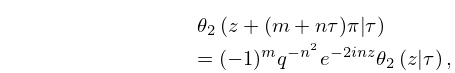
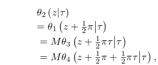
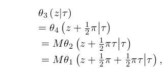
4: 20.2 Definitions and Periodic Properties

… ►

20.2.6 $${\theta }_1\left(z+(m+n\tau )\pi \right|\tau )={(-1)}^{m+n}{q}^{-n^2}{\mathrm{e}}^{-2\mathrm{i}nz}{\theta }_1\left(z\right|\tau ),$$

ⓘ

Symbols:

${\theta }_j\left(z\right|\tau )$: theta function, $\pi$: the ratio of the circumference of a circle to its diameter, $\mathrm{e}$: base of natural logarithm, $\mathrm{i}$: imaginary unit, $m$: integer, $n$: integer, $z$: complex, $\tau$: lattice parameter and $q$: nome

A&S Ref:

16.33.2 (in different notation)

Referenced by:

§23.6(i)

Permalink:

http://dlmf.nist.gov/20.2.E6

Encodings:

pMML, png, TeX

See also:

Annotations for §20.2(ii), §20.2 and Ch.20

►

20.2.7 $${\theta }_2\left(z+(m+n\tau )\pi \right|\tau )={(-1)}^m{q}^{-n^2}{\mathrm{e}}^{-2\mathrm{i}nz}{\theta }_2\left(z\right|\tau ),$$

ⓘ

Symbols:

${\theta }_j\left(z\right|\tau )$: theta function, $\pi$: the ratio of the circumference of a circle to its diameter, $\mathrm{e}$: base of natural logarithm, $\mathrm{i}$: imaginary unit, $m$: integer, $n$: integer, $z$: complex, $\tau$: lattice parameter and $q$: nome

A&S Ref:

16.33.3 (in different notation)

Permalink:

http://dlmf.nist.gov/20.2.E7

Encodings:

pMML, png, TeX

See also:

Annotations for §20.2(ii), §20.2 and Ch.20

►

20.2.8 $${\theta }_3\left(z+(m+n\tau )\pi \right|\tau )=q^{-n^2}{\mathrm{e}}^{-2\mathrm{i}nz}{\theta }_3\left(z\right|\tau ),$$

ⓘ

Symbols:

${\theta }_j\left(z\right|\tau )$: theta function, $\pi$: the ratio of the circumference of a circle to its diameter, $\mathrm{e}$: base of natural logarithm, $\mathrm{i}$: imaginary unit, $m$: integer, $n$: integer, $z$: complex, $\tau$: lattice parameter and $q$: nome

A&S Ref:

16.33.4 (in different notation)

Permalink:

http://dlmf.nist.gov/20.2.E8

Encodings:

pMML, png, TeX

See also:

Annotations for §20.2(ii), §20.2 and Ch.20

… ►

20.2.12 $${\theta }_2\left(z\right|\tau )={\theta }_1\left(z+\frac{1}{2}\pi \right|\tau )=M{\theta }_3\left(z+\frac{1}{2}\pi \tau \right|\tau )=M{\theta }_4\left(z+\frac{1}{2}\pi +\frac{1}{2}\pi \tau \right|\tau ),$$

ⓘ

Symbols:

${\theta }_j\left(z\right|\tau )$: theta function, $\pi$: the ratio of the circumference of a circle to its diameter, $z$: complex, $\tau$: lattice parameter and $M$

A&S Ref:

16.33.3 (in different notation)

Permalink:

http://dlmf.nist.gov/20.2.E12

Encodings:

pMML, png, TeX

See also:

Annotations for §20.2(iii), §20.2 and Ch.20

►

20.2.13 $${\theta }_3\left(z\right|\tau )={\theta }_4\left(z+\frac{1}{2}\pi \right|\tau )=M{\theta }_2\left(z+\frac{1}{2}\pi \tau \right|\tau )=M{\theta }_1\left(z+\frac{1}{2}\pi +\frac{1}{2}\pi \tau \right|\tau ),$$

ⓘ

Symbols:

${\theta }_j\left(z\right|\tau )$: theta function, $\pi$: the ratio of the circumference of a circle to its diameter, $z$: complex, $\tau$: lattice parameter and $M$

A&S Ref:

16.33.4 (in different notation)

Permalink:

http://dlmf.nist.gov/20.2.E13

Encodings:

pMML, png, TeX

See also:

Annotations for §20.2(iii), §20.2 and Ch.20

…

5: 18.1 Notation

… ►

$${\delta }_x\left(f(x)\right)=\left(f(x+\frac{1}{2}\mathrm{i})-f(x-\frac{1}{2}\mathrm{i})\right)/\mathrm{i},$$

…

6: 24.10 Arithmetic Properties

… ►Here and elsewhere two rational numbers are congruent if the modulus divides the numerator of their difference. …

7: 19.36 Methods of Computation

… ►The cases and require different treatment for numerical purposes, and again precautions are needed to avoid cancellations. …

8: Errata

… ►

In the online version, the leading divided difference operators were previously omitted from these formulas, due to programming error.

Reported by Nico Temme on 2021-06-01

… ►

10.22.72 $${\int }_0^{\mathrm{\infty }}{J}_{\mu }\left(at\right)J_{\nu }\left(bt\right)J_{\nu }\left(ct\right)t^{1-\mu }dt=\frac{{(bc)}^{\mu -1}\sin \left((\mu -\nu )\pi \right){(\sinh \chi )}^{\mu -\frac{1}{2}}}{{(\frac{1}{2}{\pi }^3)}^{\frac{1}{2}}{a}^{\mu }}{\mathrm{e}}^{(\mu -\frac{1}{2})\mathrm{i}\pi }{Q}_{\nu -\frac{1}{2}}^{\frac{1}{2}-\mu }\left(\cosh \chi \right),$$ $\mathrm{\Re }\mu >-\frac{1}{2},\mathrm{\Re }\nu >-1,a>b+c,\cosh \chi =(a^2-b^2-c^2)/(2bc)$

Originally, the factor on the right-hand side was written as $\frac{{(bc)}^{\mu -1}\cos \left(\nu \pi \right){(\sinh \chi )}^{\mu -\frac{1}{2}}}{{(\frac{1}{2}{\pi }^3)}^{\frac{1}{2}}{a}^{\mu }}$, which was taken directly from Watson (1944, p. 412, (13.46.5)), who uses a different normalization for the associated Legendre function of the second kind $Q_{\nu }^{\mu }$. Watson’s $Q_{\nu }^{\mu }$ equals $\frac{\sin \left((\nu +\mu )\pi \right)}{\sin \left(\nu \pi \right)}{\mathrm{e}}^{-\mu \pi \mathrm{i}}{Q}_{\nu }^{\mu }$ in the DLMF.

Reported by Arun Ravishankar on 2018-10-22

…

9: 4.24 Inverse Trigonometric Functions: Further Properties

… ►

4.24.2 $$\arccos z={(2(1-z))}^{1/2}\left(1+\sum _{n=1}^{\mathrm{\infty }}\frac{1\cdot 3\cdot 5\mathrm{\cdots }(2n-1)}{2^{2n}(2n+1)n!}{(1-z)}^n\right),$$ $|1-z|\le 2$.

ⓘ

Symbols:

$!$: factorial (as in $n!$), $\arccos z$: arccosine function, $n$: integer and $z$: complex variable

A&S Ref:

4.4.41 (which is stated differently and the constraint on $z$ is more restrictive.)

Permalink:

http://dlmf.nist.gov/4.24.E2

Encodings:

pMML, png, TeX

See also:

Annotations for §4.24(i), §4.24 and Ch.4

…

10: 7.7 Integral Representations

… ►

7.7.1 $$\mathrm{erfc}z=\frac{2}{\pi }{\mathrm{e}}^{-z^2}{\int }_0^{\mathrm{\infty }}\frac{{\mathrm{e}}^{-z^2{t}^2}}{t^2+1}dt,$$ $|\mathrm{ph}z|\le \frac{1}{4}\pi$,

ⓘ

Symbols:

$\pi$: the ratio of the circumference of a circle to its diameter, $\mathrm{erfc}z$: complementary error function, $dx$: differential of $x$ , $\mathrm{e}$: base of natural logarithm, $\int$: integral, $\mathrm{ph}$: phase and $z$: complex variable

A&S Ref:

7.4.11 (in different form)

Referenced by:

§7.11, §7.7(i)

Permalink:

http://dlmf.nist.gov/7.7.E1

Encodings:

pMML, png, TeX

See also:

Annotations for §7.7(i), §7.7 and Ch.7

… ►

7.7.7 $${\int }_x^{\mathrm{\infty }}{\mathrm{e}}^{-a^2{t}^2-(b^2/t^2)}dt=\frac{\sqrt{\pi }}{4a}\left({\mathrm{e}}^{2ab}\mathrm{erfc}\left(ax+(b/x)\right)+{\mathrm{e}}^{-2ab}\mathrm{erfc}\left(ax-(b/x)\right)\right),$$ $x>0$, .

ⓘ

Symbols:

$\pi$: the ratio of the circumference of a circle to its diameter, $\mathrm{erfc}z$: complementary error function, $dx$: differential of $x$ , $\mathrm{e}$: base of natural logarithm, $\int$: integral, $\mathrm{ph}$: phase and $x$: real variable

A&S Ref:

7.4.33 (in different form)

Referenced by:

§7.7(i), §7.8

Permalink:

http://dlmf.nist.gov/7.7.E7

Encodings:

pMML, png, TeX

See also:

Annotations for §7.7(i), §7.7 and Ch.7

►

7.7.8 $${\int }_0^{\mathrm{\infty }}{\mathrm{e}}^{-a^2{t}^2-(b^2/t^2)}dt=\frac{\sqrt{\pi }}{2a}{\mathrm{e}}^{-2ab},$$ , .

ⓘ

Symbols:

$\pi$: the ratio of the circumference of a circle to its diameter, $dx$: differential of $x$ , $\mathrm{e}$: base of natural logarithm, $\int$: integral and $\mathrm{ph}$: phase

A&S Ref:

7.4.3 (in different form)

Referenced by:

§7.7(i)

Permalink:

http://dlmf.nist.gov/7.7.E8

Encodings:

pMML, png, TeX

See also:

Annotations for §7.7(i), §7.7 and Ch.7

… ►

7.7.10 $$\mathrm{f}\left(z\right)=\frac{1}{\pi \sqrt{2}}{\int }_0^{\mathrm{\infty }}\frac{{\mathrm{e}}^{-\pi z^{2}t/2}}{\sqrt{t}(t^2+1)}dt,$$ $|\mathrm{ph}z|\le \frac{1}{4}\pi$,

ⓘ

Symbols:

$\mathrm{f}\left(z\right)$: auxiliary function for Fresnel integrals, $\pi$: the ratio of the circumference of a circle to its diameter, $dx$: differential of $x$ , $\mathrm{e}$: base of natural logarithm, $\int$: integral, $\mathrm{ph}$: phase and $z$: complex variable

A&S Ref:

7.4.26 (in different form)

Referenced by:

§7.12(ii), §7.7(ii)

Permalink:

http://dlmf.nist.gov/7.7.E10

Encodings:

pMML, png, TeX

See also:

Annotations for §7.7(ii), §7.7 and Ch.7

►

7.7.11 $$\mathrm{g}\left(z\right)=\frac{1}{\pi \sqrt{2}}{\int }_0^{\mathrm{\infty }}\frac{\sqrt{t}{\mathrm{e}}^{-\pi z^{2}t/2}}{t^2+1}dt,$$ $|\mathrm{ph}z|\le \frac{1}{4}\pi$,

ⓘ

Symbols:

$\mathrm{g}\left(z\right)$: auxiliary function for Fresnel integrals, $\pi$: the ratio of the circumference of a circle to its diameter, $dx$: differential of $x$ , $\mathrm{e}$: base of natural logarithm, $\int$: integral, $\mathrm{ph}$: phase and $z$: complex variable

A&S Ref:

7.4.25 (in different form)

Referenced by:

§7.12(ii), §7.7(ii)

Permalink:

http://dlmf.nist.gov/7.7.E11

Encodings:

pMML, png, TeX

See also:

Annotations for §7.7(ii), §7.7 and Ch.7

…