boundary conditions and the Weyl alternative

♦ 1—10 of 36 matching pages ♦

(0.003 seconds)

1—10 of 36 matching pages

1: 1.18 Linear Second Order Differential Operators and Eigenfunction Expansions

… ►

Self-adjoint extensions of (1.18.28) and the Weyl alternative

…

2: 3.6 Linear Difference Equations

… ►However,

w_{n}

can be computed successfully in these circumstances by boundary-value methods, as follows. … ►For a difference equation of order

k

(

\geq 3

), …or for systems of

k

first-order inhomogeneous equations, boundary-value methods are the rule rather than the exception. Typically

k-\ell

conditions are prescribed at the beginning of the range, and

\ell

conditions at the end. …

3: 1.6 Vectors and Vector-Valued Functions

… ►

§1.6(ii) Vectors: Alternative Notations

… ►Note: The terminology open and closed sets and boundary points in the

(x,y)

plane that is used in this subsection and §1.6(v) is analogous to that introduced for the complex plane in §1.9(ii). … ►and

S

be the closed and bounded point set in the

(x,y)

plane having a simple closed curve

C

as boundary. … ►Suppose

S

is an oriented surface with boundary

\,\partial S

which is oriented so that its direction is clockwise relative to the normals of

S

. …

4: 32.11 Asymptotic Approximations for Real Variables

… ►Next, for given initial conditions

w(0)=0

and

w^{\prime}(0)=k

, with

k

real,

w(x)

has at least one pole on the real axis. … ►with boundary condition … ►and with boundary condition … ►Alternatively, if

\nu

is not zero or a positive integer, then …

5: Bibliography L

… ►

D. Lemoine (1997) Optimal cylindrical and spherical Bessel transforms satisfying bound state boundary conditions. Comput. Phys. Comm. 99 (2-3), pp. 297–306.

ⓘ

Notes:: Single-precision Fortran, maximum accuracy 8S.
External Links:: ISSN 0010-4655, Document, Code, ZentralBlatt
Referenced by:: 4th item.
Encodings:: BibTeX

… ►

H. A. Lorentz, A. Einstein, H. Minkowski, and H. Weyl (1923) The Principle of Relativity: A Collection of Original Memoirs on the Special and General Theory of Relativity. Methuen and Co., Ltd., London.

ⓘ

Notes:: Translated from Das Relativitätsprinzip by W. Perrett and G. B. Jeffery. Reprinted by Dover Publications Inc., New York, 1952.
External Links:: MathReview, ZentralBlatt
Referenced by:: §1.6(ii).
Encodings:: BibTeX

…

6: 32.2 Differential Equations

… ►In general the singularities of the solutions are movable in the sense that their location depends on the constants of integration associated with the initial or boundary conditions. … ►

§32.2(iii) Alternative Forms

…

7: 34.2 Definition: $\mathit{3j}$ Symbol

… ►They therefore satisfy the triangle conditions … ►If either of the conditions (34.2.1) or (34.2.3) is not satisfied, then the

\mathit{3j}

symbol is zero. When both conditions are satisfied the

\mathit{3j}

symbol can be expressed as the finite sum … ►

34.2.6

\begin{pmatrix}j_{1}&j_{2}&j_{3}\\ m_{1}&m_{2}&m_{3}\end{pmatrix}={(-1)^{j_{2}-m_{1}+m_{3}}}\frac{(j_{1}+j_{2}+m_% {3})!(j_{2}+j_{3}-m_{1})!}{\Delta(j_{1}j_{2}j_{3})(j_{1}+j_{2}+j_{3}+1)!}\left% (\frac{(j_{1}+m_{1})!(j_{3}-m_{3})!}{(j_{1}-m_{1})!(j_{2}+m_{2})!(j_{2}-m_{2})% !(j_{3}+m_{3})!}\right)^{\frac{1}{2}}\*{{{}_{3}F_{2}}\left(-j_{1}-j_{2}-j_{3}-% 1,-j_{1}+m_{1},-j_{3}-m_{3};-j_{1}-j_{2}-m_{3},-j_{2}-j_{3}+m_{1};1\right)},

ⓘ

Symbols:: ${{}_{\NVar{p}}F_{\NVar{q}}}\left(\NVar{a_{1},\dots,a_{p}};\NVar{b_{1},\dots,b_% {q}};\NVar{z}\right)$ or ${{}_{\NVar{p}}F_{\NVar{q}}}\left({\NVar{a_{1},\dots,a_{p}}\atop\NVar{b_{1},% \dots,b_{q}}};\NVar{z}\right)$ : alternatively ${{}_{\NVar{p}}F_{\NVar{q}}}\left(\NVar{\mathbf{a}};\NVar{\mathbf{b}};\NVar{z}\right)$ or ${{}_{\NVar{p}}F_{\NVar{q}}}\left({\NVar{\mathbf{a}}\atop\NVar{\mathbf{b}}};% \NVar{z}\right)$
generalized hypergeometric function, $!$ : factorial (as in $n!$ ), $\begin{pmatrix}\NVar{j_{1}}&\NVar{j_{2}}&\NVar{j_{3}}\\ \NVar{m_{1}}&\NVar{m_{2}}&\NVar{m_{3}}\end{pmatrix}$ : $\mathit{3j}$ symbol, $j,j_{r}$ : non-negative integers or non-negative integers plus one half. and $\Delta(j_{1}j_{2}j_{3})$ : product
Referenced by:: §18.38(iii)
Permalink:: http://dlmf.nist.gov/34.2.E6
Encodings:: pMML, png, TeX
See also:: Annotations for §34.2 and Ch.34

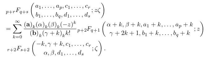
… ►For alternative expressions for the

\mathit{3j}

symbol, written either as a finite sum or as other terminating generalized hypergeometric series

{{}_{3}F_{2}}

of unit argument, see Varshalovich et al. (1988, §§8.21, 8.24–8.26).

8: 1.10 Functions of a Complex Variable

… ►Let

D

be a bounded domain with boundary

\partial D

and let

\overline{D}=D\cup\partial D

. … ►(Or more generally, a simple contour that starts at the center and terminates on the boundary.) … ►Alternatively, take

z_{0}

to be any point in

D

and set

F(z_{0})={\mathrm{e}}^{\alpha\ln\left(1-z_{0}\right)}{\mathrm{e}}^{\beta\ln% \left(1+z_{0}\right)}

where the logarithms assume their principal values. … ►This result is also true when

b=\infty

, or when

f(z,t)

has a singularity at

t=b

, with the following conditions. … ►The last condition means that given

\epsilon

(

>0

) there exists a number

a_{0}\in[a,b)

that is independent of

z

and is such that …

9: 21.9 Integrable Equations

… ►These parameters, including

\boldsymbol{{\Omega}}

, are not free: they are determined by a compact, connected Riemann surface (Krichever (1976)), or alternatively by an appropriate initial condition

u(x,y,0)

(Deconinck and Segur (1998)). …

10: 16.10 Expansions in Series of ${{}_{p}F_{q}}$ Functions

… ►The following expansion, with appropriate conditions and together with similar results, is given in Fields and Wimp (1961): ►

16.10.1

{{}_{p+r}F_{q+s}}\left({a_{1},\dots,a_{p},c_{1},\dots,c_{r}\atop b_{1},\dots,b% _{q},d_{1},\dots,d_{s}};z\zeta\right)=\sum_{k=0}^{\infty}\frac{{\left(\mathbf{% a}\right)_{k}}{\left(\alpha\right)_{k}}{\left(\beta\right)_{k}}(-z)^{k}}{{% \left(\mathbf{b}\right)_{k}}{\left(\gamma+k\right)_{k}}k!}{{}_{p+2}F_{q+1}}% \left({\alpha+k,\beta+k,a_{1}+k,\dots,a_{p}+k\atop\gamma+2k+1,b_{1}+k,\dots,b_% {q}+k};z\right){{}_{r+2}F_{s+2}}\left({-k,\gamma+k,c_{1},\dots,c_{r}\atop% \alpha,\beta,d_{1},\dots,d_{s}};\zeta\right).

ⓘ

Symbols:: ${{}_{\NVar{p}}F_{\NVar{q}}}\left(\NVar{a_{1},\dots,a_{p}};\NVar{b_{1},\dots,b_% {q}};\NVar{z}\right)$ or ${{}_{\NVar{p}}F_{\NVar{q}}}\left({\NVar{a_{1},\dots,a_{p}}\atop\NVar{b_{1},% \dots,b_{q}}};\NVar{z}\right)$ : alternatively ${{}_{\NVar{p}}F_{\NVar{q}}}\left(\NVar{\mathbf{a}};\NVar{\mathbf{b}};\NVar{z}\right)$ or ${{}_{\NVar{p}}F_{\NVar{q}}}\left({\NVar{\mathbf{a}}\atop\NVar{\mathbf{b}}};% \NVar{z}\right)$
generalized hypergeometric function, ${\left(\NVar{a}\right)_{\NVar{n}}}$ : Pochhammer’s symbol (or shifted factorial), $!$ : factorial (as in $n!$ ), $p$ : nonnegative integer, $q$ : nonnegative integer, $z$ : complex variable, $a,a_{1},\ldots,a_{p}$ : real or complex parameters and $b,b_{1},\ldots,b_{q}$ : real or complex parameters
Permalink:: http://dlmf.nist.gov/16.10.E1
Encodings:: pMML, png, TeX
See also:: Annotations for §16.10 and Ch.16

… ►

16.10.2

{{}_{p+1}F_{p}}\left({a_{1},\dots,a_{p+1}\atop b_{1},\dots,b_{p}};z\zeta\right% )=(1-z)^{-a_{1}}\sum_{k=0}^{\infty}\frac{{\left(a_{1}\right)_{k}}}{k!}{{}_{p+1% }F_{p}}\left({-k,a_{2},\dots,a_{p+1}\atop b_{1},\dots,b_{p}};\zeta\right)\left% (\frac{z}{z-1}\right)^{k}.

ⓘ

Symbols:: ${{}_{\NVar{p}}F_{\NVar{q}}}\left(\NVar{a_{1},\dots,a_{p}};\NVar{b_{1},\dots,b_% {q}};\NVar{z}\right)$ or ${{}_{\NVar{p}}F_{\NVar{q}}}\left({\NVar{a_{1},\dots,a_{p}}\atop\NVar{b_{1},% \dots,b_{q}}};\NVar{z}\right)$ : alternatively ${{}_{\NVar{p}}F_{\NVar{q}}}\left(\NVar{\mathbf{a}};\NVar{\mathbf{b}};\NVar{z}\right)$ or ${{}_{\NVar{p}}F_{\NVar{q}}}\left({\NVar{\mathbf{a}}\atop\NVar{\mathbf{b}}};% \NVar{z}\right)$
generalized hypergeometric function, ${\left(\NVar{a}\right)_{\NVar{n}}}$ : Pochhammer’s symbol (or shifted factorial), $!$ : factorial (as in $n!$ ), $p$ : nonnegative integer, $z$ : complex variable, $a,a_{1},\ldots,a_{p}$ : real or complex parameters and $b,b_{1},\ldots,b_{q}$ : real or complex parameters
Permalink:: http://dlmf.nist.gov/16.10.E2
Encodings:: pMML, png, TeX
See also:: Annotations for §16.10 and Ch.16

…