bifurcation%20set

SearchAdvancedHelp

(0.002 seconds)

21—30 of 606 matching pages

21: 7.23 Tables

… ►

Abramowitz and Stegun (1964, Chapter 7) includes $\mathrm{erf}x$, $(2/\sqrt{\pi }){\mathrm{e}}^{-x^2}$, $x\in [0,2]$, 10D; $(2/\sqrt{\pi }){\mathrm{e}}^{-x^2}$, $x\in [2,10]$, 8S; $x{\mathrm{e}}^{x^2}\mathrm{erfc}x$, $x^{-2}\in [0,0.25]$, 7D; $2^n\mathrm{\Gamma }\left(\frac{1}{2}n+1\right){\mathrm{i}}^n\mathrm{erfc}\left(x\right)$, $n=1(1)6,10,11$, $x\in [0,5]$, 6S; $F\left(x\right)$, $x\in [0,2]$, 10D; $xF\left(x\right)$, $x^{-2}\in [0,0.25]$, 9D; $C\left(x\right)$, $S\left(x\right)$, $x\in [0,5]$, 7D; $\mathrm{f}\left(x\right)$, $\mathrm{g}\left(x\right)$, $x\in [0,1]$, $x^{-1}\in [0,1]$, 15D.

… ►

Zhang and Jin (1996, pp. 637, 639) includes $(2/\sqrt{\pi }){\mathrm{e}}^{-x^2}$, $\mathrm{erf}x$, $x=0(.02)1(.04)3$, 8D; $C\left(x\right)$, $S\left(x\right)$, $x=0(.2)10(2)100(100)500$, 8D.

… ►

Zhang and Jin (1996, pp. 638, 640–641) includes the real and imaginary parts of $\mathrm{erf}z$, $x\in [0,5]$, $y=0.5(.5)3$, 7D and 8D, respectively; the real and imaginary parts of ${\int }_x^{\mathrm{\infty }}{\mathrm{e}}^{\pm \mathrm{i}{t}^2}dt$, $(1/\sqrt{\pi }){\mathrm{e}}^{\mp \mathrm{i}(x^2+(\pi /4))}{\int }_x^{\mathrm{\infty }}{\mathrm{e}}^{\pm \mathrm{i}{t}^2}dt$, $x=0(.5)20(1)25$, 8D, together with the corresponding modulus and phase to 8D and 6D (degrees), respectively.

…

22: 8.26 Tables

… ►

Khamis (1965) tabulates $P(a,x)$ for $a=0.05(.05)10(.1)20(.25)70$, $0.0001\le x\le 250$ to 10D.

… ►

Abramowitz and Stegun (1964, pp. 245–248) tabulates $E_n\left(x\right)$ for $n=2,3,4,10,20$, $x=0(.01)2$ to 7D; also $(x+n){\mathrm{e}}^x{E}_n\left(x\right)$ for $n=2,3,4,10,20$, $x^{-1}=0(.01)0.1(.05)0.5$ to 6S.

… ►

Pagurova (1961) tabulates $E_n\left(x\right)$ for $n=0(1)20$, $x=0(.01)2(.1)10$ to 4-9S; ${\mathrm{e}}^x{E}_n\left(x\right)$ for $n=2(1)10$, $x=10(.1)20$ to 7D; ${\mathrm{e}}^x{E}_p\left(x\right)$ for $p=0(.1)1$, $x=0.01(.01)7(.05)12(.1)20$ to 7S or 7D.

… ►

Zhang and Jin (1996, Table 19.1) tabulates $E_n\left(x\right)$ for $n=1,2,3,5,10,15,20$, $x=0(.1)1,1.5,2,3,5,10,20,30,50,100$ to 7D or 8S.

23: 23 Weierstrass Elliptic and Modular
Functions

…

24: 5.22 Tables

… ►Abramowitz and Stegun (1964, Chapter 6) tabulates $\mathrm{\Gamma }\left(x\right)$, $\ln \mathrm{\Gamma }\left(x\right)$, $\psi \left(x\right)$, and ${\psi }^{\prime }\left(x\right)$ for $x=1(.005)2$ to 10D; ${\psi }^{\prime \prime }\left(x\right)$ and ${\psi }^{(3)}\left(x\right)$ for $x=1(.01)2$ to 10D; $\mathrm{\Gamma }\left(n\right)$, $1/\mathrm{\Gamma }\left(n\right)$, $\mathrm{\Gamma }\left(n+\frac{1}{2}\right)$, $\psi \left(n\right)$, ${\log }_{10}\mathrm{\Gamma }\left(n\right)$, ${\log }_{10}\mathrm{\Gamma }\left(n+\frac{1}{3}\right)$, ${\log }_{10}\mathrm{\Gamma }\left(n+\frac{1}{2}\right)$, and ${\log }_{10}\mathrm{\Gamma }\left(n+\frac{2}{3}\right)$ for $n=1(1)101$ to 8–11S; $\mathrm{\Gamma }\left(n+1\right)$ for $n=100(100)1000$ to 20S. Zhang and Jin (1996, pp. 67–69 and 72) tabulates $\mathrm{\Gamma }\left(x\right)$, $1/\mathrm{\Gamma }\left(x\right)$, $\mathrm{\Gamma }\left(-x\right)$, $\ln \mathrm{\Gamma }\left(x\right)$, $\psi \left(x\right)$, $\psi \left(-x\right)$, ${\psi }^{\prime }\left(x\right)$, and ${\psi }^{\prime }\left(-x\right)$ for $x=0(.1)5$ to 8D or 8S; $\mathrm{\Gamma }\left(n+1\right)$ for $n=0(1)100(10)250(50)500(100)3000$ to 51S. …

25: 26.10 Integer Partitions: Other Restrictions

… ► $p(\in S,n)$ denotes the number of partitions of $n$ into parts taken from the set $S$. The set $\{n\ge 1|n\equiv \pm j(modk)\}$ is denoted by $A_{j,k}$. The set $\{2,3,4,\mathrm{\dots }\}$ is denoted by $T$. … ►

26.10.14 $$p(𝒟2,\in T,n)=p(\in A_{2,5},n),$$ $T=\{2,3,4,\mathrm{\dots }\}$,

ⓘ

Symbols:

$\in$: element of, $p(\mathrm{condition},n)$: restricted number of partitions of $n$ , $n$: nonnegative integer, $A_{j,k}$: set and $T$: set

Referenced by:

§26.10(iv)

Permalink:

http://dlmf.nist.gov/26.10.E14

Encodings:

pMML, png, TeX

See also:

Annotations for §26.10(iv), §26.10 and Ch.26

… ►

26.10.16 $$p(𝒟,n)\sim \frac{{\mathrm{e}}^{\pi \sqrt{n/3}}}{{(768n^3)}^{1/4}},$$ $n\to \mathrm{\infty }$.

ⓘ

Symbols:

$\sim$: asymptotic equality, $\pi$: the ratio of the circumference of a circle to its diameter, $\mathrm{e}$: base of natural logarithm, $p(\mathrm{condition},n)$: restricted number of partitions of $n$ and $n$: nonnegative integer

A&S Ref:

24.2.2

Permalink:

http://dlmf.nist.gov/26.10.E16

Encodings:

pMML, png, TeX

See also:

Annotations for §26.10(v), §26.10 and Ch.26

…

26: 3.8 Nonlinear Equations

… ►(More precisely, $p$ is the largest of the possible set of indices for (3.8.3).) … ►Consider $x=20$ and $j=19$. We have $p^{\prime }(20)=19!$ and $a_{19}=1+2+\mathrm{\cdots }+20=210$. … ►It is called a Julia set. In general the Julia set of an analytic function $f(z)$ is a fractal, that is, a set that is self-similar. …

27: 6.16 Mathematical Applications

… ►Hence if $x=\pi /(2n)$ and $n\to \mathrm{\infty }$, then the limiting value of $S_n(x)$ overshoots $\frac{1}{4}\pi$ by approximately 18%. Similarly if $x=\pi /n$, then the limiting value of $S_n(x)$ undershoots $\frac{1}{4}\pi$ by approximately 10%, and so on. … ►

►►

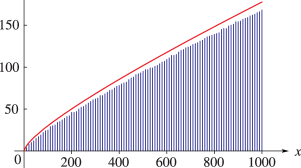
Figure 6.16.2: The logarithmic integral $\mathrm{li}\left(x\right)$, together with vertical bars indicating the value of $\pi (x)$ for $x=10,20,\mathrm{\dots },1000$. Magnify

28: 32.8 Rational Solutions

… ►

32.8.3 $$w(z;3)=\frac{3z^2}{z^3+4}-\frac{6z^2(z^3+10)}{z^6+20z^3-80},$$

ⓘ

Symbols:

$z$: real

Permalink:

http://dlmf.nist.gov/32.8.E3

Encodings:

pMML, png, TeX

See also:

Annotations for §32.8(ii), §32.8 and Ch.32

►

32.8.4 $$w(z;4)=-\frac{1}{z}+\frac{6z^2(z^3+10)}{z^6+20z^3-80}-\frac{9z^5(z^3+40)}{z^9+60z^6+11200}.$$

ⓘ

Symbols:

$z$: real

Permalink:

http://dlmf.nist.gov/32.8.E4

Encodings:

pMML, png, TeX

See also:

Annotations for §32.8(ii), §32.8 and Ch.32

… ►

$$Q_3(z)=z^6+20z^3-80,$$

… ►In the general case assume $\gamma \delta \ne 0$, so that as in §32.2(ii) we may set $\gamma =1$ and $\delta =-1$. … ►In the general case assume $\delta \ne 0$, so that as in §32.2(ii) we may set $\delta =-\frac{1}{2}$. …

29: 7.8 Inequalities

… ►

7.8.2 $x\ge 0$,

ⓘ

Symbols:

$𝖬\left(x\right)$: Mills’ ratio, $\pi$: the ratio of the circumference of a circle to its diameter and $x$: real variable

A&S Ref:

7.1.13

Referenced by:

§7.8

Permalink:

http://dlmf.nist.gov/7.8.E2

Encodings:

pMML, png, TeX

See also:

Annotations for §7.8 and Ch.7

… ►

7.8.5 $x\ge 0$.

ⓘ

Symbols:

$𝖬\left(x\right)$: Mills’ ratio and $x$: real variable

Referenced by:

§7.8

Permalink:

http://dlmf.nist.gov/7.8.E5

Encodings:

pMML, png, TeX

See also:

Annotations for §7.8 and Ch.7

… ►The function $F\left(x\right)/\sqrt{1-{\mathrm{e}}^{-2x^2}}$ is strictly decreasing for $x>0$. … ►

7.8.8 $x>0$.

ⓘ

Symbols:

$\pi$: the ratio of the circumference of a circle to its diameter, $\mathrm{erf}z$: error function, $\mathrm{e}$: base of natural logarithm and $x$: real variable

Source:

Pólya (1949, (1.5))

Referenced by:

§7.8, Erratum (V1.0.17) for Equation (7.8.8)

Permalink:

http://dlmf.nist.gov/7.8.E8

Encodings:

pMML, png, TeX

Addition (effective with 1.0.17):

This inequality was added. It is Pólya (1949, (1.5)). Note that it is a special case of (8.10.11).

Suggested by Roberto Iacono

See also:

Annotations for §7.8 and Ch.7

30: 11.14 Tables

… ►

Zhang and Jin (1996) tabulates ${𝐇}_n\left(x\right)$ and ${𝐋}_n\left(x\right)$ for $n=-4(1)3$ and $x=0(1)20$ to 8D or 7S.

… ►

Abramowitz and Stegun (1964, Chapter 12) tabulates ${\int }_0^x(I_0\left(t\right)-{𝐋}_0\left(t\right))dt$ and $(2/\pi ){\int }_x^{\mathrm{\infty }}{t}^{-1}{𝐇}_0\left(t\right)dt$ for $x=0(.1)5$ to 5D or 7D; ${\int }_0^x({𝐇}_0\left(t\right)-Y_0\left(t\right))dt-(2/\pi )\ln x$, ${\int }_0^x(I_0\left(t\right)-{𝐋}_0\left(t\right))dt-(2/\pi )\ln x$, and ${\int }_x^{\mathrm{\infty }}{t}^{-1}({𝐇}_0\left(t\right)-Y_0\left(t\right))dt$ for $x^{-1}=0(.01)0.2$ to 6D.

…