Verblunsky coefficients

SearchAdvancedHelp

(0.002 seconds)

11—20 of 241 matching pages

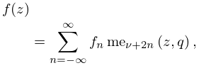
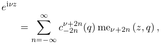
11: 28.19 Expansions in Series of ${\mathrm{me}}_{\nu +2n}$ Functions

… ►

28.19.2 $$f(z)=\sum _{n=-\mathrm{\infty }}^{\mathrm{\infty }}{f}_n{\mathrm{me}}_{\nu +2n}(z,q),$$

ⓘ

Defines:

$f(z)$: function (locally)

Symbols:

${\mathrm{me}}_n(z,q)$: Mathieu function, $q=h^2$: parameter, $n$: integer, $z$: complex variable, $\nu$: complex parameter and $f_n$: coefficients

Referenced by:

§28.19

Permalink:

http://dlmf.nist.gov/28.19.E2

Encodings:

pMML, png, TeX

See also:

Annotations for §28.19 and Ch.28

… ►

28.19.3 $$f_n=\frac{1}{\pi }{\int }_0^{\pi }f(z){\mathrm{me}}_{\nu +2n}(-z,q)dz.$$

ⓘ

Defines:

$f_n$: coefficients (locally)

Symbols:

${\mathrm{me}}_n(z,q)$: Mathieu function, $\pi$: the ratio of the circumference of a circle to its diameter, $dx$: differential of $x$ , $\int$: integral, $q=h^2$: parameter, $n$: integer, $z$: complex variable, $\nu$: complex parameter and $f(z)$: function

Permalink:

http://dlmf.nist.gov/28.19.E3

Encodings:

pMML, png, TeX

See also:

Annotations for §28.19 and Ch.28

… ►

28.19.4 $${\mathrm{e}}^{\mathrm{i}\nu z}=\sum _{n=-\mathrm{\infty }}^{\mathrm{\infty }}{c}_{-2n}^{\nu +2n}(q){\mathrm{me}}_{\nu +2n}(z,q),$$

ⓘ

Symbols:

${\mathrm{me}}_n(z,q)$: Mathieu function, $\mathrm{e}$: base of natural logarithm, $\mathrm{i}$: imaginary unit, $q=h^2$: parameter, $n$: integer, $z$: complex variable, $\nu$: complex parameter and $c_{2m}(q)$: coefficients

Permalink:

http://dlmf.nist.gov/28.19.E4

Encodings:

pMML, png, TeX

See also:

Annotations for §28.19, §28.19 and Ch.28

►where the coefficients are as in §28.14.

12: 26.16 Multiset Permutations

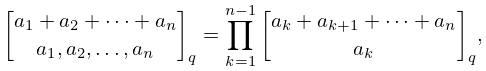
… ►The number of elements in ${𝔖}_S$ is the multinomial coefficient (§26.4) $\left(\genfrac{}{}{0.0pt}{}{a_1+a_2+\mathrm{\cdots }+a_n}{a_1,a_2,\mathrm{\dots },a_n}\right)$. … ►Thus $inv(351322453154)=4+8+0+3+1+1+2+3+1+0+1=24$, and $maj(351322453154)=2+4+8+9+11=34.$ ►The $q$-multinomial coefficient is defined in terms of Gaussian polynomials (§26.9(ii)) by ►

26.16.1 $${\left[\genfrac{}{}{0.0pt}{}{a_1+a_2+\mathrm{\cdots }+a_n}{a_1,a_2,\mathrm{\dots },a_n}\right]}_q=\prod _{k=1}^{n-1}{\left[\genfrac{}{}{0.0pt}{}{a_k+a_{k+1}+\mathrm{\cdots }+a_n}{a_k}\right]}_q,$$

ⓘ

Symbols:

${\left[\genfrac{}{}{0.0pt}{}{n}{m}\right]}_q$: $q$-binomial coefficient (or Gaussian polynomial), ${\left[\genfrac{}{}{0.0pt}{}{a_1+a_2+\mathrm{\cdots }+a_n}{a_1,a_2,\mathrm{\dots },a_n}\right]}_q$: $q$-multinomial coefficient, $k$: nonnegative integer, $n$: nonnegative integer, $a_j$: numbers and $q$: parameter

Permalink:

http://dlmf.nist.gov/26.16.E1

Encodings:

pMML, png, TeX

See also:

Annotations for §26.16 and Ch.26

… ►

26.16.2 $$\sum _{\sigma \in {𝔖}_S}{q}^{inv(\sigma )}={\left[\genfrac{}{}{0.0pt}{}{a_1+a_2+\mathrm{\cdots }+a_n}{a_1,a_2,\mathrm{\dots },a_n}\right]}_q,$$

ⓘ

Symbols:

$\in$: element of, ${\left[\genfrac{}{}{0.0pt}{}{a_1+a_2+\mathrm{\cdots }+a_n}{a_1,a_2,\mathrm{\dots },a_n}\right]}_q$: $q$-multinomial coefficient, ${𝔖}_n$: set of permutations of $\{1,2,\mathrm{\dots },n\}$ , $n$: nonnegative integer, $a_j$: numbers, $S$: multiset and $q$: parameter

Permalink:

http://dlmf.nist.gov/26.16.E2

Encodings:

pMML, png, TeX

See also:

Annotations for §26.16 and Ch.26

…

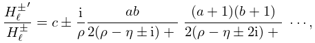
13: 33.8 Continued Fractions

… ►

33.8.2 $$\frac{H_{\mathrm{\ell }}^{\pm }{}_{}{}^{\prime }}{H_{\mathrm{\ell }}^{\pm }}=c\pm \frac{\mathrm{i}}{\rho }\frac{ab}{2(\rho -\eta \pm \mathrm{i})+}\frac{(a+1)(b+1)}{2(\rho -\eta \pm 2\mathrm{i})+}\mathrm{\cdots },$$

ⓘ

Symbols:

$\mathrm{i}$: imaginary unit, $H_{\mathrm{\ell }}^{\pm }(\eta ,\rho )$: irregular Coulomb radial functions, $\mathrm{\ell }$: nonnegative integer, $\rho$: nonnegative real variable, $\eta$: real parameter, $a$: coefficient, $b$: coefficient and $c$: coefficient

Referenced by:

§33.8

Permalink:

http://dlmf.nist.gov/33.8.E2

Encodings:

pMML, png, TeX

See also:

Annotations for §33.8 and Ch.33

…

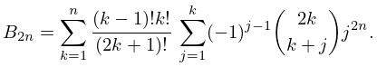
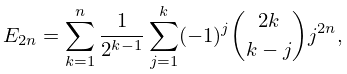
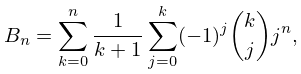
14: 24.6 Explicit Formulas

… ►

24.6.1 $$B_{2n}=\sum _{k=2}^{2n+1}\frac{{(-1)}^{k-1}}{k}\left(\genfrac{}{}{0pt}{}{2n+1}{k}\right)\sum _{j=1}^{k-1}{j}^{2n},$$

ⓘ

Symbols:

$B_n$: Bernoulli numbers, $\left(\genfrac{}{}{0.0pt}{}{m}{n}\right)$: binomial coefficient, $j$: integer, $k$: integer and $n$: integer

Referenced by:

§24.6

Permalink:

http://dlmf.nist.gov/24.6.E1

Encodings:

pMML, png, TeX

See also:

Annotations for §24.6 and Ch.24

►

24.6.2 $$B_n=\frac{1}{n+1}\sum _{k=1}^n\sum _{j=1}^k{(-1)}^j{j}^n\left(\genfrac{}{}{0.0pt}{}{n+1}{k-j}\right)/\left(\genfrac{}{}{0.0pt}{}{n}{k}\right),$$

ⓘ

Symbols:

$B_n$: Bernoulli numbers, $\left(\genfrac{}{}{0.0pt}{}{m}{n}\right)$: binomial coefficient, $j$: integer, $k$: integer and $n$: integer

Referenced by:

§24.6

Permalink:

http://dlmf.nist.gov/24.6.E2

Encodings:

pMML, png, TeX

See also:

Annotations for §24.6 and Ch.24

►

24.6.3 $$B_{2n}=\sum _{k=1}^n\frac{(k-1)!k!}{(2k+1)!}\sum _{j=1}^k{(-1)}^{j-1}\left(\genfrac{}{}{0pt}{}{2k}{k+j}\right)j^{2n}.$$

ⓘ

Symbols:

$B_n$: Bernoulli numbers, $\left(\genfrac{}{}{0.0pt}{}{m}{n}\right)$: binomial coefficient, $!$: factorial (as in $n!$), $j$: integer, $k$: integer and $n$: integer

Referenced by:

§24.6

Permalink:

http://dlmf.nist.gov/24.6.E3

Encodings:

pMML, png, TeX

See also:

Annotations for §24.6 and Ch.24

►

24.6.4 $$E_{2n}=\sum _{k=1}^n\frac{1}{2^{k-1}}\sum _{j=1}^k{(-1)}^j\left(\genfrac{}{}{0pt}{}{2k}{k-j}\right)j^{2n},$$

ⓘ

Symbols:

$E_n$: Euler numbers, $\left(\genfrac{}{}{0.0pt}{}{m}{n}\right)$: binomial coefficient, $j$: integer, $k$: integer and $n$: integer

Referenced by:

§24.6

Permalink:

http://dlmf.nist.gov/24.6.E4

Encodings:

pMML, png, TeX

See also:

Annotations for §24.6 and Ch.24

… ►

24.6.9 $$B_n=\sum _{k=0}^n\frac{1}{k+1}\sum _{j=0}^k{(-1)}^j\left(\genfrac{}{}{0pt}{}{k}{j}\right)j^n,$$

ⓘ

Symbols:

$B_n$: Bernoulli numbers, $\left(\genfrac{}{}{0.0pt}{}{m}{n}\right)$: binomial coefficient, $j$: integer, $k$: integer and $n$: integer

Referenced by:

§24.6

Permalink:

http://dlmf.nist.gov/24.6.E9

Encodings:

pMML, png, TeX

See also:

Annotations for §24.6 and Ch.24

…

15: 20.6 Power Series

… ►Here the coefficients are given by ►

20.6.6 $${\delta }_{2j}(\tau )=\sum _{n=-\mathrm{\infty }}^{\mathrm{\infty }}\sum _{\begin{array}{c}m=-\mathrm{\infty }\\ \left|m\right|+\left|n\right|\ne 0\end{array}}^{\mathrm{\infty }}{(m+n\tau )}^{-2j},$$

ⓘ

Defines:

${\delta }_{2j}(\tau )$: coefficient (locally)

Symbols:

$m$: integer, $n$: integer and $\tau$: lattice parameter

Referenced by:

§20.6, §20.6

Permalink:

http://dlmf.nist.gov/20.6.E6

Encodings:

pMML, png, TeX

See also:

Annotations for §20.6 and Ch.20

►

20.6.7 $${\alpha }_{2j}(\tau )=\sum _{n=-\mathrm{\infty }}^{\mathrm{\infty }}\sum _{m=-\mathrm{\infty }}^{\mathrm{\infty }}{(m-\frac{1}{2}+n\tau )}^{-2j},$$

ⓘ

Defines:

${\alpha }_{2j}(\tau )$: coefficient (locally)

Symbols:

$m$: integer, $n$: integer and $\tau$: lattice parameter

Permalink:

http://dlmf.nist.gov/20.6.E7

Encodings:

pMML, png, TeX

See also:

Annotations for §20.6 and Ch.20

►

20.6.8 $${\beta }_{2j}(\tau )=\sum _{n=-\mathrm{\infty }}^{\mathrm{\infty }}\sum _{m=-\mathrm{\infty }}^{\mathrm{\infty }}{(m-\frac{1}{2}+(n-\frac{1}{2})\tau )}^{-2j},$$

ⓘ

Defines:

${\beta }_{2j}(\tau )$: coefficient (locally)

Symbols:

$m$: integer, $n$: integer and $\tau$: lattice parameter

Referenced by:

§20.6

Permalink:

http://dlmf.nist.gov/20.6.E8

Encodings:

pMML, png, TeX

See also:

Annotations for §20.6 and Ch.20

►

20.6.9 $${\gamma }_{2j}(\tau )=\sum _{n=-\mathrm{\infty }}^{\mathrm{\infty }}\sum _{m=-\mathrm{\infty }}^{\mathrm{\infty }}{(m+(n-\frac{1}{2})\tau )}^{-2j},$$

ⓘ

Defines:

${\gamma }_{2j}(\tau )$: coefficient (locally)

Symbols:

$m$: integer, $n$: integer and $\tau$: lattice parameter

Permalink:

http://dlmf.nist.gov/20.6.E9

Encodings:

pMML, png, TeX

See also:

Annotations for §20.6 and Ch.20

…

16: 2.9 Difference Equations

… ►Often $f(n)$ and $g(n)$ can be expanded in series …Formal solutions are … ► $c_0=1$, and higher coefficients are determined by formal substitution. … ►with $a_{0,j}=1$ and higher coefficients given by (2.9.7) (in the present case the coefficients of $a_{s,j}$ and $a_{s-1,j}$ are zero). … ►The coefficients $b_s$ and constant $c$ are again determined by formal substitution, beginning with $c=1$ when ${\alpha }_2-{\alpha }_1=0$, or with $b_0=1$ when ${\alpha }_2-{\alpha }_1=1,2,3,\mathrm{\dots }$. …

17: Errata

… ►In regard to orthogonal polynomials on the unit circle, we now discuss monic polynomials, Verblunsky’s Theorem, and Szegő’s theorem. … ►

A sentence indicating that explicit representations for the coefficients $c_k$ are given in Volkmer (2023) was inserted just below (16.11.5).

… ►

Equations: (3.3.3_1), (3.3.3_2), (5.15.9) (suggested by Calvin Khor on 2021-09-04), (8.15.2), Pochhammer symbol representation in (10.17.1) for $a_k(\nu )$ coefficient, Pochhammer symbol representation in (11.9.4) for $a_k(\mu ,\nu )$ coefficient, and (12.14.4_5).

… ►

The reference for Clebsch-Gordan coefficients, Condon and Shortley (1935), was replaced by Edmonds (1974) and Rotenberg et al. (1959). The references for $\mathit{3}j$, $\mathit{6}j$, $\mathit{9}j$ symbols were made more precise.

… ►

10.20.14 $$B_3(0)=-\frac{\mathrm{959\hspace{0.33em}71711\hspace{0.33em}84603}}{\mathrm{25\hspace{0.33em}47666\hspace{0.33em}37125\hspace{0.33em}00000}}{2}^{\frac{1}{3}}$$

Originally this coefficient was given incorrectly as $B_3(0)=-\frac{\mathrm{430\hspace{0.33em}99056\hspace{0.33em}39368\hspace{0.33em}59253}}{\mathrm{5\hspace{0.33em}68167\hspace{0.33em}34399\hspace{0.33em}42500\hspace{0.33em}00000}}{2}^{\frac{1}{3}}$. The other coefficients in this equation have not been changed.

Reported 2012-05-11 by Antony Lee.

…

18: 16.24 Physical Applications

… ►

§16.24(iii) $\mathit{3}j$, $\mathit{6}j$, and $\mathit{9}j$ Symbols

►The $\mathit{3}j$ symbols, or Clebsch–Gordan coefficients, play an important role in the decomposition of reducible representations of the rotation group into irreducible representations. …The coefficients of transformations between different coupling schemes of three angular momenta are related to the Wigner $\mathit{6}j$ symbols. …

19: 33.20 Expansions for Small $|ϵ|$

… ►where ►

33.20.4 $${𝖥}_k(\mathrm{\ell };r)=\sum _{p=2k}^{3k}{(2r)}^{(p+1)/2}{C}_{k,p}{J}_{2\mathrm{\ell }+1+p}\left(\sqrt{8r}\right),$$ $r>0$,

ⓘ

Symbols:

$J_{\nu }\left(z\right)$: Bessel function of the first kind, $k$: nonnegative integer, $\mathrm{\ell }$: nonnegative integer, $r$: real variable, ${𝖥}_k(\mathrm{\ell };r)$: coefficient and $C_{k,p}$: coefficients

Permalink:

http://dlmf.nist.gov/33.20.E4

Encodings:

pMML, png, TeX

See also:

Annotations for §33.20(ii), §33.20 and Ch.33

… ►The functions $J$ and $I$ are as in §§10.2(ii), 10.25(ii), and the coefficients $C_{k,p}$ are given by $C_{0,0}=1$, $C_{1,0}=0$, and … ►where $A(ϵ,\mathrm{\ell })$ is given by (33.14.11), (33.14.12), and …The functions $Y$ and $K$ are as in §§10.2(ii), 10.25(ii), and the coefficients $C_{k,p}$ are given by (33.20.6). …

20: 18.22 Hahn Class: Recurrence Relations and Differences

… ►

18.22.2 $$-x{p}_n(x)=A_n{p}_{n+1}(x)-\left(A_n+C_n\right)p_n(x)+C_n{p}_{n-1}(x),$$

ⓘ

Symbols:

$p_n(x)$: polynomial of degree $n$ , $n$: nonnegative integer, $x$: real variable, $A_n$: coefficient and $C_n$: coefficient

Referenced by:

§16.4(iii), §18.21(ii), §18.22(i), Table 18.22.1

Permalink:

http://dlmf.nist.gov/18.22.E2

Encodings:

pMML, png, TeX

See also:

Annotations for §18.22(i), §18.22(i), §18.22 and Ch.18

… ►

18.22.5 $$(a+\mathrm{i}x)q_n(x)={\tilde{A}}_n{q}_{n+1}(x)-\left({\tilde{A}}_n+{\tilde{C}}_n\right)q_n(x)+{\tilde{C}}_n{q}_{n-1}(x),$$

ⓘ

Symbols:

$\mathrm{i}$: imaginary unit, $n$: nonnegative integer, $x$: real variable, ${\tilde{A}}_n$: coefficient and ${\tilde{C}}_n$: coefficient

Permalink:

http://dlmf.nist.gov/18.22.E5

Encodings:

pMML, png, TeX

See also:

Annotations for §18.22(i), §18.22(i), §18.22 and Ch.18

… ►

18.22.10 $$A(x)p_n(x+1)-\left(A(x)+C(x)\right)p_n(x)+C(x)p_n(x-1)-n(n+\alpha +\beta +1)p_n(x)=0,$$

ⓘ

Symbols:

$p_n(x)$: polynomial of degree $n$ , $n$: nonnegative integer, $x$: real variable, $A(x)$: coefficient and $C(x)$: coefficient

Referenced by:

§16.4(iii)

Permalink:

http://dlmf.nist.gov/18.22.E10

Encodings:

pMML, png, TeX

See also:

Annotations for §18.22(ii), §18.22(ii), §18.22 and Ch.18

… ►

18.22.12 $$A(x)p_n(x+1)-\left(A(x)+C(x)\right)p_n(x)+C(x)p_n(x-1)+{\lambda }_n{p}_n(x)=0.$$

ⓘ

Symbols:

$p_n(x)$: polynomial of degree $n$ , $n$: nonnegative integer, $x$: real variable, $C(x)$: coefficient, ${\lambda }_n$: coefficient and $A(x)$: coefficient

Referenced by:

§18.22(ii), Table 18.22.2

Permalink:

http://dlmf.nist.gov/18.22.E12

Encodings:

pMML, png, TeX

See also:

Annotations for §18.22(ii), §18.22(ii), §18.22 and Ch.18

… ►

18.22.14 $$A(x)p_n(x+\mathrm{i})-\left(A(x)+C(x)\right)p_n(x)+C(x)p_n(x-\mathrm{i})+n(n+2\mathrm{\Re }\left(a+b\right)-1)p_n(x)=0,$$

ⓘ

Symbols:

$\mathrm{i}$: imaginary unit, $\mathrm{\Re }$: real part, $p_n(x)$: polynomial of degree $n$ , $n$: nonnegative integer, $x$: real variable, $A(x)$: coefficient and $C(x)$: coefficient

Referenced by:

§18.22(ii), §18.22(iii)

Permalink:

http://dlmf.nist.gov/18.22.E14

Encodings:

pMML, png, TeX

See also:

Annotations for §18.22(ii), §18.22(ii), §18.22 and Ch.18

…